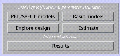
This section deals with the specification of a model to analyse imaging data, and subsequent parameter estimation. Statistical inference is performed using the Results option (see 4). SPM distinguishes three classes of models:
For modality-specific, independent data (PET/SPECT models; 3.1).
For modality-specific, serially correlated data (fMRI models, 3.2).
Basic models for independent data, which include random effects (RFX) analyses (3.3).
3.1 PET/SPECT models (spm_spm_ui.m)
SPM offers a number of PET/SPECT prototype models, which limits the number of necessary specifications for easy use.
N.B.
All data entered in the model need to be in the same position (i.e., coregistered), and have identical dimensions and voxel sizes.
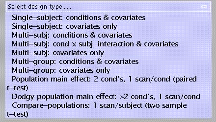
Single-subject, conditions & covariates: e.g. analysis of an individual subject, 12 scans (ARARARARARAR), with habituation (time) as a covariate. See example 1 below
Single-subject, covariates only: e.g., analysis of an individual subject, 12 scans during which a task is performed, with covariate = task score (this example is discussed in Matthew Brett's tutorial on SPM statistics; see http://www.mrc-cbu.cam.ac.uk/Imaging/spmstats.html )
Multi-subject, conditions & covariates: e.g., a study with 10 subjects, each performing a task with three levels of difficulty, with reaction time as a covariate (i.e, a condition x covariate interaction)
Multi-subject, condition x subject interaction & covariates: conditions are modelled separately for each subject, which allows assessment of condition x subject interactions. See example 2 below
Multi-subject, covariates only: e.g., a study with 6 spider phobic patients shown slides of spiders during each of 12 scans, with anxiety ratings as a covariate
Multi-group: conditions & covariates: e.g., a factorial design with two groups of subjects both performing an ARARARARARAR experiment. This design allows assessment of main effects (task vs. rest) for each group separately and both groups combined, as well as task x group interaction effects
Multi-group, covariates only: e.g., the 'Multi-subject, covariates only' spider study with a group of non-phobic controls added
Population main effect: 2 conditions, 1 scan/condition (= modality-adjusted paired t-test), e.g., a PET or SPECT study using a dopaminergic ligand in subjects with Parkinson's disease scanned both pre- and post-therapy
Dodgy population main effect: > 2 conditions, 1 scan/condition; 'dodgy' because sphericity assumptions are likely to be violated (see example 1 below)
Compare-populations: 1 condition, 1 scan/condition (=modality-adjusted two-sample t-test), e.g., a PET or SPECT ligand study comparing patients to normal controls
Compare-populations (AnCova): 1 condition, 1 scan/condition, with nuisance variable(s) added, e.g. the preceding study with age entered as a possible confound
The Full Monty: 'asks you everything'; an amalgam of 'Multi-subject, cond x subj interaction & covariates' and 'Multi-group' options
Example 1: single-subject: conditions & covariates
Select:
![]()
Specify a vector whose length equals the number of scans, e.g. 1 2 1 2 1 2 1 2 1 2 1 2:
![]()
Specify:
![]()
If a covariate is modelled, specify a vector whose length also equals the number of scans:
![]()
Specify (e.g., time):
![]()
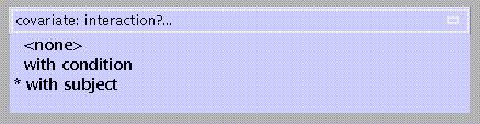
Specify:
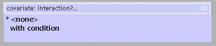
'none' will model the covariate (=time) as one parameter (time x session) or column in the design matrix (see below); 'with condition' as two (time x cond1 and time x cond2).
Specify:
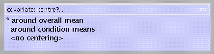
Centring a covariate ensures that main effects of the interacting factor are not affected by the covariate, therefore SPM suggests centring on the overall mean. If 'interaction by condition' had been specified, the default becomes 'centring around condition means'.
Specify:
![]()
(=0 in this example; otherwise, specification of nuisance variables is similar to covariates).
Specify:
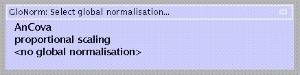
Scan to scan differences in global flow can be:
modelled as a nuisance variable (AnCova),
adjusted for by scaling the voxel values for each scan to the mean (proportional scaling)
ignored.
AnCova is advised for multi-subject studies unless differences in global flow are large (e.g., due to variability in injected tracer dose). Because AnCova also uses one degree of freedom for each subject/group, proportional scaling may be preferable for single-subject studies.
If proportional scaling is selected, specify:
![]()
the default of which scales the global flow to a physiologically realistic value of 50 ml/dl/min.
Specify:
![]()
to ensure that only grey-matter voxels are included in the analysis, by masking out from all scans voxels that fail to reach the specified threshold.
If 'proportional' is selected, specify:
![]()
the default being 80% of the mean global value. If thresholding is to be omitted, specify '-Inf'.
Specify:
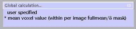
The default is a two-step process in which first the overall mean is computed, after which voxels which do not reach a threshold of overall mean/8 (i.e., those which are extra-cranial) get masked out, followed by a second computation of the mean of the remaining voxels.
Output from PET/SPECT models (spm_spm_ui) for example 1:
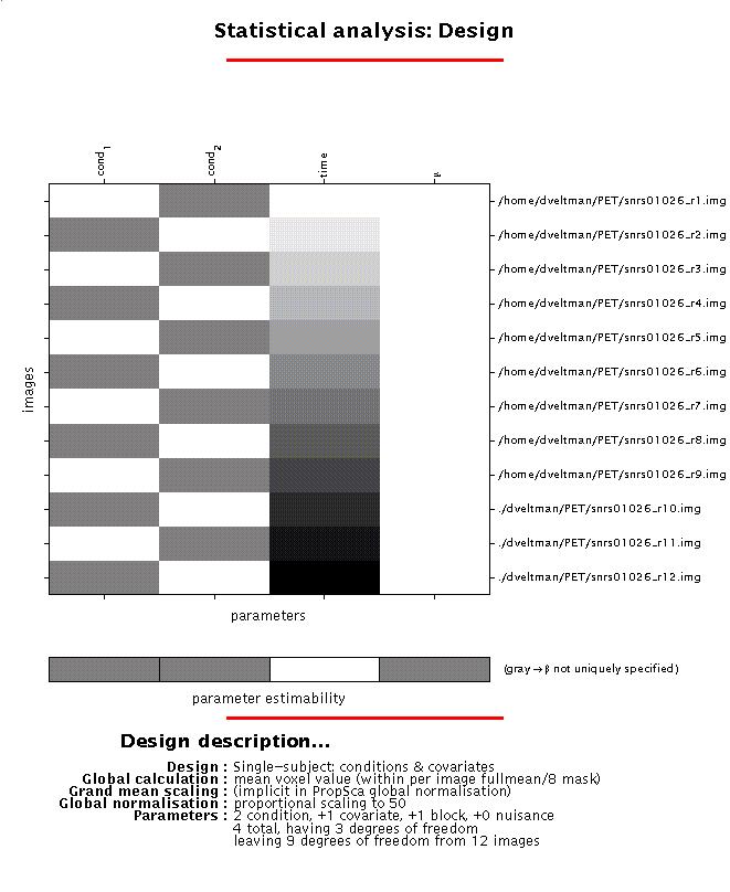
Display: SPM displays a design matrix having columns for each parameter (in this example, two conditions, one covariate, and one constant (block)) and a row for each scan. The grey-and-white bar below the design matrix signals that the matrix is rank deficient (columns 1,2 and 4 are linearly dependent) which limits selection of meaningful contrasts (parameter weights) for condition effects to those which sum up to zero (see 4).
File: the design matrix will be saved as SPMcfg.mat in the working directory.
Specify:
![]()
to begin parameter estimation now or at a later stage. If 'later', select 'Estimate' (middle panel) and select the appropriate SPMcfg.mat file.
Example 2: Multi-subject, cond x subj interaction & covariates.
Consider a study in which five subjects perform an attention task with two stimulus types alternated with rest (ABRABRABRABR, suitably randomised across subjects) where individual differences in arousal (measured as skin conductance (GSR)) may interact with performance.
Specify (5):
![]()
Select:
![]()
Specify (for each subject) a vector whose length equals the number of scans, e.g. A B R R A B B R A A R B:
![]()
Specify (1):
![]()
Specify a vector whose length equals the total number of scans:
![]()
Specify (GSR):
![]()
Specify (with subject):
'none' will model the covariate (=GSR) as one parameter (GSR x session) or column in the design matrix (see below); 'with condition' as three (GSR x cond1-3) and 'with subject ' as five (GSR x subj1-5).
Specify:
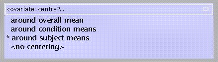
Centring a covariate ensures that main effects of the interacting factor are not affected by the covariate, therefore SPM here suggests centring on subject means.
Specify (0):
![]()
Select:
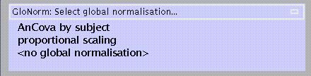
Scan to scan differences in global flow can be:
modelled as a nuisance variable (AnCova),
adjusted for by scaling the voxel values for each scan to the mean (proportional scaling)
ignored.
AnCova is advised for multi-subject studies unless differences in global flow are large (e.g., due to variability in injected tracer dose). Because AnCova also uses one degree of freedom for each subject/group, proportional scaling may be preferable for single-subject studies.
If AnCova is selected, specify:
the default corrects for subject to subject differences in mean global flow (within-subject differences were modelled during the previous step).
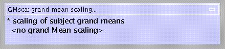
Specify (50):
![]()
the default of which scales the global flow to a physiologically realistic value of 50 ml/dl/min.
As in example 1, specify:
![]()
to ensure that only grey-matter voxels are included in the analysis, by masking out voxels which fail to reach the specified threshold.
If 'proportional' is selected, specify:
![]()
the default being 80% of the mean global value. If thresholding is to be omitted, specify '-Inf'.
Specify:

the default is a two-step process in which first the overall mean is computed, after which voxels which do not reach a threshold of overall mean/8 (i.e. extracranial voxels) get masked out, followed by a second computation of the mean of the remaining voxels.
Output from PET/SPECT models (spm_spm_ui) for example 2:
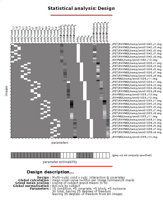
Display: SPM displays a design matrix having columns for each parameter (in this example, fifteen conditions (three conditions, modelled separately for each subject), one covariate (GSR for each subject), five constants (block) and five nuisance variables (GBF)), and a row for each scan. The grey-and-white bar below the design matrix signals that the matrix is rank deficient (columns 1-15 and 21-25 are linearly dependent) which limits selection of meaningful contrasts (parameter weights) for condition effects to those which sum up to zero (see 4).
File: the design matrix will be saved as SPMcfg.mat in the working directory.
As in example 1, specify:
![]()
to begin parameter estimation now or at a later stage. If 'later', select 'Estimate' (middle panel) and select the appropriate SPMcfg.mat file.
N.B.
Model estimation may also be launched via the 'Explore design' option. SPM will then prompt you to select a SPMcfg.mat file for inspection.
Clicking 'Design' (lower left window) will activate a pull-down menu which allows selection of displays for the design matrix, details of design orthogonality (surfable), selected scans and specified conditions, and covariates. It does not provide options to edit the model.
Output from PET/SPECT parameter estimation (spm_spm.m):
beta_0001.img/hdr, beta_0002.img/hdr, beta_0003.img/hdr, ?.. : images containing parameter estimates for each column in the design matrix
mask.hdr/img : mask image consisting of 0's and 1's indicating which voxels within the image volume are to be assessed
ResMS.hdr/img : image of estimated residual variance
RPV.hdr/img : image of estimated resels per voxel
SPM.mat file : contains details of design matrix, analysed images, search volume, smoothness estimates and results files.
xCon.mat file : contains default F-contrast (so-called 'effects of interest') which are used for selecting 'interesting' voxels at which to save raw data for future plotting
Y.mad file : contains (in compressed form) the raw (unsmoothed) data at voxels with an F-statistic higher than the default. Each column corresponds to one voxel, each row to an input image
Yidx.mat file : contains a 1 x N vector of column indices used in the Y.mad file (where N = number of available voxels)
3.2 fMRI models (spm_fmri_spm_ui.m)
3.2.1 Specification of a model - first step:
Select 'specify a model':
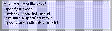
As with PET/SPECT, SPM'99 allows separate model specification & inspection, and parameter estimation, for fMRI designs. However, fMRI model building is more flexible, the main distinction being between epoch- and event-related designs.
N.B.
Whereas model specification & parameter estimation occurs in two stages for PET/SPECT studies, for fMRI there are three:
specification of conditions, timings, user-specified covariates, and regressor types (e.g. boxcar),
selecting scans, modelling nuisance variables and other confounds, i.e. low-frequency drifts and temporal autocorrelation,
parameter estimation. This permits the use of a single design matrix (i.e., the first step) for different data sets (sessions/subjects) acquired with the same paradigm, and also for designing an experiment (stochastic designs, see below). In SPM, the first step is termed 'specify a model', the second and third 'estimate a specified model'.
In the 'specify and estimate a model' option, the order of the prompts is slightly different; moreover, SPM does not display graphs of the specified regressor(s) and design orthogonality (these can be displayed using the 'review a specified model' option and selecting the appropriate SPM_fMRIDesMtx.mat file).
Specify:
N.B.
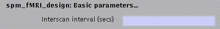
As with PET/SPECT, all data entered in the model need to be in the same position (i.e., coregistered), and have identical dimensions and voxel sizes.
In addition, the TR must be identical.
Specify:
![]()
Here SPM does not distinguish between sessions and subjects: e.g., for a design with 4 subjects each having two sessions of 96 scans, enter 96 96 96 96 96 96 96 96.
When more than one session is entered, specify:
![]()
If 'no', SPM will prompt for the number (and names) of conditions / trials for each session. If 'yes', specify:
![]()
If 'no' (as will be usually the case, i.e. when replications are randomised across sessions), SPM will prompt for onset times/trial lengths for each session.
Specify:
![]()
for all sessions combined when conditions are replicated, or otherwise for each session separately.
Specify:
![]()
for each condition.
Specify:
![]()
This option allows building an (event-related) experiment rather than analysing one. If 'yes', SPM will prompt to specify:
Whether to include a null event,
Whether there is a fixed time delay between consecutive events of the same type (SOA, see below),
The relative frequency of event types (e.g., 1/1),
Whether this frequency should be stationary or modulated across the experiment.
The resulting design matrix can be used for both conducting and analysing an experiment. Otherwise, select 'no'.
Specify:
![]()
if 'fixed', specify:
![]()
SOA = stimulus onset asynchrony = time (in scans) between the onset of two consecutive appearances of the same condition/trial type. This must be entered for each trial/condition.
Specify:
![]()
for each trial/condition. For example, if the1st trial occurs at the beginning of the first scan, enter 0, if it occurs halfway through the 3rd scan, enter 2.5.
If SOA = 'variable', specify:
![]()
again for each trial/condition. Enter the onset in scans for each occurrence of the trial. The length of this vector should equal the number of times the trial occurs (replications).
Next, specify:
![]()
and if yes, specify trial durations for each replication:
![]()
Again, the length of this vector should equal the number of trials (4 in this example).
N.B.
SOA = stimulus onset asynchrony = time (in scans) between the onset of two consecutive appearances of the same condition/trial type. As an example, consider a time series of 96 scans with conditions A, B, and R, each block lasting 8 scans; if the scanning order is ABRABRABRABR, SOA = fixed (24 scans), onset time = 0/8/16 for A/B/R. If the scanning order is randomised to ABRRBABARRAB, SOA = variable, vector of onsets = 0 40 56 80/8 32 48 88/16 24 64 72 for A/B/R.
If block lengths within a condition are different, it should be analysed as an event-related design (see below). Alternatively, it can be specified as an epoch design with separate conditions for each block length. For example, consider a simple ARAR? study in which condition A alternately lasts 7 or 8 scans; this can be modelled as A1RA2R? where A1 = 7-scan activation blocks, and A2 = 8-scan activation blocks.
In these examples, a resting condition is included for clarity. A resting condition (baseline) need not be explicitly modelled in SPM, however.
Specify:
![]()
This option allows modelling changes over replications of conditions/trials across session.
If 'time' or 'other', select:
![]()
to model linear, exponential, or polynomial changes. (When choosing 'polynomial', SPM will prompt for the order of the polynomial, the default being 2 generating a polynomial with linear + squared components).
Next, specify condition or trial numbers in which a parametric term should be included (e.g. for 2 trials, select 1, 2 or both):
![]()
If 'other', SPM will also prompt for a vector whose length is equal to the number of replications (e.g., 10):
For two or more condition/trial types, specify:
![]()
For each condition, trials should be either events or epochs. If mixed, SPM prompts to specify 'events' or 'epochs' for each condition separately. If there is only one condition, SPM will also prompt to specify 'events' or 'epochs'.
For an epoch design, select:
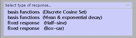
i.e., a function or set of functions which, convolved with the timings specified earlier, provides the most adequate modelling of the data. Basis functions are more flexible than fixed response models but their components usually cannot be interpreted in a physiologically meaningful way; therefore multivariate or F-contrasts are required for statistical inference (see 4). A discrete cosine set may be useful when a steady-state response does not occur; SPM will prompt for the number of functions (default = 2). Similarly, mean & exponential decay may be chosen when the response decreases over time within an epoch (as opposed to across replications, see above).
Next, select:
![]()
Convolving with the canonical hemodynamic response function (hrf) will add a delayed onset, early peak, and late undershoot to the model.
Select:
![]()
if yes, the partial derivative of e.g. the boxcar function with respect to time is added as an additional regressor, which will enable modelling of slight onset differences.
Finally, specify for each condition modelled as epochs:
![]()
For an event-related design, select:
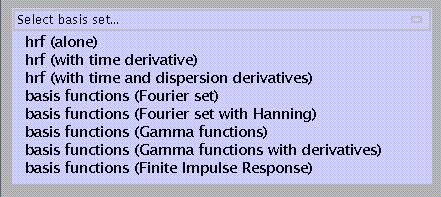
hrf (alone): canonical hemodynamic response function; based on empirical (visual stimulation) data; consists of two gamma functions (one positive, one negative) shifted 2s apart.
hrf (with time derivative): hrf with partial derivative for time added; allows modelling of slight (ca. 1s) onset differences.
hrf (with time and dispersion derivatives): hrf with partial derivatives for time and dispersion added; allows modelling of slight onset differences in onset time and response width.
basis functions (Fourier set): uses a set of sines/cosines to model responses. The default window length is 32s (at which time the canonical hrf has returned to baseline), the default number of functions is 4, resulting in 9 basis functions: sines/cosines with frequency 1/32, 2/32, 3/32 and 4/32 Hz, and a constant. The number of functions should be chosen with regard to the TR, as it is doubtful whether one should include components higher than the Nyquist frequency (i.e., 1/(2TR) Hz).
basis functions (Fourier set with Hanning): similar to the previous option but with an amplitude modulation (Hanning filter) added so that all functions start and end at zero.
basis functions (Gamma functions): uses three gamma functions (which are asymmetrical) with different onset-to-peak times and orthogonalised with respect to each other.
basis functions (Gamma functions with derivatives): similar to the previous option but with temporal derivatives for each function added.
basis functions (Finite Impulse Response): uses a set of 'mini-boxcars' to model peri-stimulus time. The default bin size (= 'boxcar length') is 2s, the default number of bins is 8, giving 9 functions (1 constant).
N.B.
As with epoch designs, basis functions are more flexible (no prior assumptions regarding the shape of the response, especially the Fourier and FIR sets) but their components cannot be interpreted in a physiologically meaningful way and therefore usually need F-contrasts for inference.
When T-contrasts are required (e.g., for a second-level analysis, see 3.3 and 4), hrf with or without time and dispersion derivatives should be chosen.
For both epoch and event-related designs, specify:
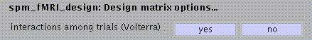
This option allows modelling (regressing out) of non-linearities due to the interaction of successive trials of the same type (for example, repetition suppression (priming)). Use also when the time between successive events is 2s or less.
Specify:
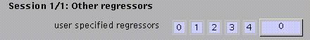
to model any other covariates (i.e., other than modulation across replications (e.g., time) or within a block (=mean and exponential decay, see above)). SPM will prompt for a vector whose length equals the number of scans (e.g., 64):
![]()
Output from fMRI model specification (spm_fmri_spm_ui.m) - first step:
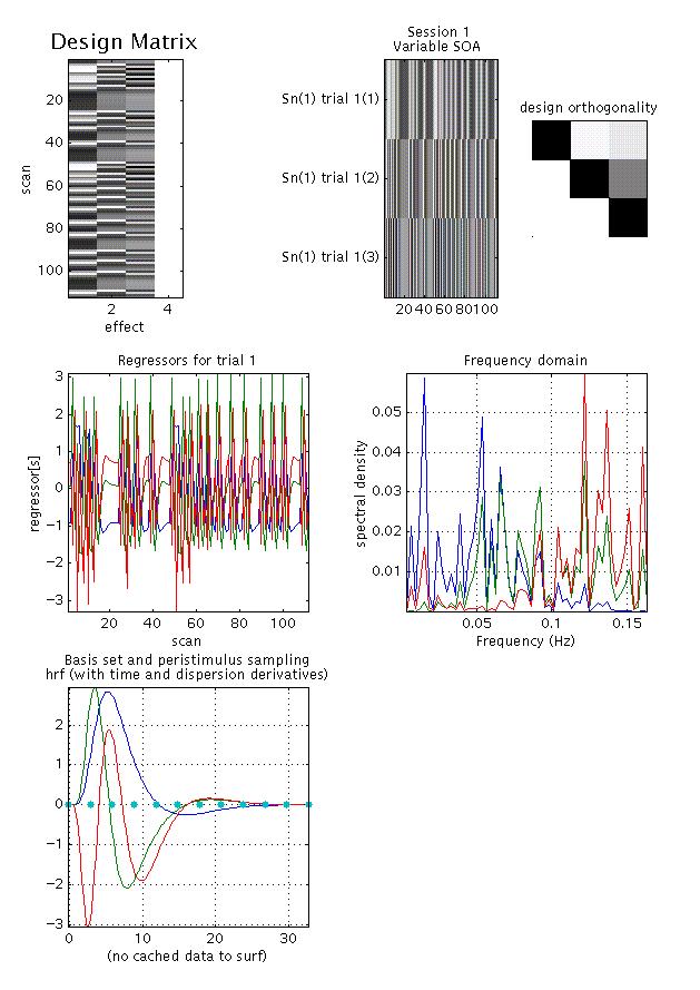
Display: shown for an event-related design, 112 scans, one event type, modelled using a canonical hrf with time and dispersion derivatives. There are six panels:
upper left: shows the columns in the design matrix, one for each regressor, one constant (block). This matrix is surfable: R-clicking will show parameter names, L-clicking will show design matrix values for each scan
upper middle: shows the 'columns' of the previous graph (except for the constant) after a 90° rotation, giving a 'bar graph' showing positive (light grey -white) and negative (dark grey - black) values across session for regressor(s) used
upper right: graph of design orthogonality: white = orthogonal, black = collinear, grey = between orthogonal and collinear. This matrix is also surfable: L-clicking will give the value of the cosine of the angle between two parameters (0 = orthogonal, 1 = collinear)
middle left: shows a more detailed graph of each regressor across session (cf. upper middle panel)
middle right: shows a Fourier (frequency domain) transform of each regressor
lower: shows a graph of each regressor relative to peri-stimulus sampling (time bins)
N.B.
As shown in this example, the regressors are not completely orthogonal due to the limited number of sampling points (orthogonality therefore varies with TR length).
File: the output of fMRI model specification at this point is saved as SPM_fMRIDesMtx.mat in the working directory.
N.B.
SPM displays only the first trial/session. To review the model for subsequent trials/sessions, select 'review a model' from 'fMRI models', select the SPM_fMRIDesMtx.mat file, and click 'Explore fMRI design' (lower left window), which will activate a pull-down menu.
3.2.2 Specification of a model - second step:
To complete specification and proceed to estimating your model, select estimate a specified model from 'fMRI models':

Select:
![]()
Select scans (for each session/subject):
![]()
Specify:
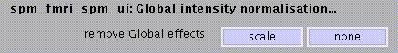
which provides the option of scaling global activity within a session (scaling across sessions/subjects occurs implicitly). This may remove e.g. scanner drifts within a session; on the other hand, large activations may be scaled down as well.
Specify:
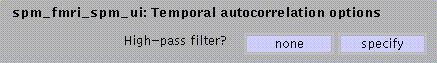
Select specify if low-frequency confounds are to be removed.
![]() :
:
The default suggested by SPM for epoch designs is two times the experimental cycle, e.g., for an ARAR?. design with A=8 scans and R=6, the default cut-off is 2(8+6)*TR. For event-related designs, the default is two times the longest interval between two appearances of the most frequently occurring event. For both epoch- and event-related designs the lower threshold is 32sec, the upper threshold is 512sec.
Specify:
![]()
If there were no correction for temporal autocorrelation in fMRI data, statistical inference would produce inflated results (the actual number of degrees of freedom is lower than the number of observations (scans)). SPM99 gives two options to deal with this problem:
Replacing the unknown autocorrelations by an imposed autocorrelation structure, by smoothing the data with a temporal filter that will attenuate high frequency components, hence a 'low-pass filter'. The shape of this filter can be either Gaussian or hrf. Differences between these two are slight but hrf may provide a better sensitivity for event-related data modelled using a hrf-basis function;
Attempting to regress out the unknown autocorrelations (AR(1)-model, see below).
If Gaussian, specify filter width (default = 4sec):
![]()
A large (wide) filter implies that attenuation will occur at lower frequencies (or, put differently, that high frequencies will be suppressed more) than with a small filter. The trade-off is that a large filter may remove interesting data while a small filter will not be adequate to impose a new (known) autocorrelation structure on the data.
Specify:
![]()
AR(1) = auto-regression (1) = modelling serial correlations by regressing out the variance explained by the previous observation (scan).
N.B.
Either temporal smoothing or AR(1) should be chosen, not both.
It is unclear whether the AR(1) option provides adequate correction for serial correlations and hence biased statistics. More extensive autoregression models (AR(n)) are more flexible than low-pass filtering but are computationally demanding.
Serial correlations affect only statistical inference at the first level. Correction may therefore be omitted when one is only interested in a second-level (random effects) analysis.
Finally, specify:
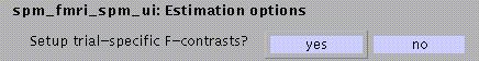
i.e., default F-contrasts for each trial type will be computed.
Output from fMRI model specification (spm_fmri_spm_ui.m) - 2nd step:

Display: the design matrix shown at this point is simply the left upper panel of the previous graph, with the file names of the scans added, and with other details of the configuration listed underneath.
Output: the configuration for the design matrix is saved as SPMcgf.mat in the working directory.
N.B.
The design matrix is also shown when the 'specify and estimate a model' option has been chosen.
As with PET/SPECT models, SPM provides the option to begin parameter estimation now or at a later stage:
![]()
If 'later', select 'Estimate' (middle panel) and select the appropriate SPMcfg.mat file.
N.B.
Model estimation may also be launched via the 'Explore design' option. SPM will prompt you to select a SPMDesMtx.mat or a SPMcfg.mat file for inspection.
Clicking 'Design' (lower left window) will activate a pull-down menu that allows selection of displays for the design matrix for each session, details of design orthogonality (surfable), and model estimation (when the SPMcfg.mat file was selected).
Output from fMRI parameter estimation (spm_spm.m):
beta_0001.img/hdr, beta_0002.img/hdr, beta_0003.img/hdr, ?.. : images containing parameter estimates for each column in the design matrix
mask.hdr/img : mask image consisting of 0's and 1's indicating which voxels within the image volume are to be assessed
ResMS.hdr/img : image of estimated residual variance
RPV.hdr/img : image of estimated resels per voxel
SPM.mat: contains details of design matrix, analysed images, search volume, smoothness estimates and results files.
xCon.mat: contains default F-contrast (so-called 'effects of interest') which are used for selecting 'interesting' voxels at which to save raw data for future plotting
Y.mad: contains (in compressed form) the raw (unsmoothed) data at voxels with an F-statistic higher than the default. Each column corresponds to one voxel, each row to an input image
Yidx.mat: contains a 1 x N vector of column indices used in the Y.mad file (where N = number of available voxels)
3.3 Customisations for PET/SPECT and fMRI statistics
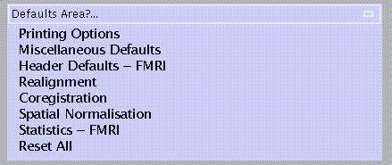
Select PET or fMRI statistics from the lower panel:
Defaults for model specification and parameter estimation are few to allow maximal flexibility.
For both PET and fMRI, specify:
![]()
for the default 'effects of interest'-F-test. The default value for PET is p<0.05 uncorrected (for multiple comparisons), for fMRI p<0.001 uncorrected.
For fMRI only, specify:
![]()
SPM interpolates each TR over this number of time bins to increase temporal resolution. 16 is chosen as default because it provides a reasonable degree of temporal resolution for typical TRs of 3-4s. The number of time bins could be equal to the number of slices, but increasing this number will not gain any real sensitivity (with typical TRs, given the time constants of the HRF and temporal smoothing), and may slow down computation.
Specify:
![]()
SPM uses the sampled bin to determine the value of a covariate at each scan. This should be adjusted if slice time correction is selected (e.g. for event-related fMRI) and the middle slice in time has been chosen as a reference slice (see 2.4). In this case, if the number of bins is 16, the sampled bin should =8 (i.e. the corresponding middle time bin).
3.4 Basic models (spm.spm_ui.m)
These are basic models for simple statistics, usually at a second level to extend the sphere of inference (random effects (RFX) analysis). Because SPM considers only a single component of variance (the residual error of variance), all analyses involving repeated measures within subjects are to be considered fixed-effects analyses, so that inferences are only valid for the sample under study. To allow inferences valid for the population from which the sample was drawn, a two-stage analysis is required, to account for first or intrasubject and second or between-subject levels of variance. During the first step, scan to scan variance (intrasubject) is modelled for each subject separately, resulting in a summary measure or 'scan'. These summary scans (usually t-contrast images (con*.img), containing weighted parameter estimates; see 4) are then fed into a second, between-subjects level analysis, using the 'Basic models' option.
N.B.
For second-level analyses, first-level individual subject models should be the same (i.e. it should be a balanced design).
To compute contrast images for a second-level analysis, either a single-subject OR a subject-separable multi-subject model should be chosen for the first level analysis, i.e. for PET 'Multi-subject, cond x subj interaction & covariates' (single-group design) or 'Full Monty' (multi-group design).
For fMRI, each subject should be specified as one session, or contrasts should be specified over sessions. For example, if 10 subjects did two sessions each, this can be analysed as a 20-session experiment, with individual contrast images specified by 1 1 0 0 0 ?., 0 0 1 1 0 ?.., and so forth.
The 'Basic models' option may also be used to analyse 'raw' (first-level) data. For this purpose SPM provides options for global normalisation, grand mean scaling and thresholding / implicit masking similar to those discussed for PET/SPECT models. For second-level analyses, however, it is not necessary to use these options at this stage because global normalisation etc. has been specified as part of the first level analysis.
Select:
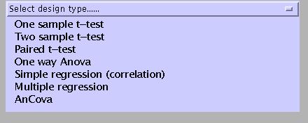
One sample t-test: tests the null hypothesis that the mean of one group of observations is identical to zero. For example, a second level analysis of activation-rest contrast images from a multi-subject experiment.
Two sample t-test: tests the null hypothesis that the mean of one group of observations is identical to the mean of a second group of observations. For example, a second level analysis of activation-rest contrast images from a two-group (e.g., patients and controls) experiment.
Paired t-test: tests the null hypothesis that the mean difference between a group of paired observations is zero. For example, a second level analysis of activation-rest contrast images from a multi-subject experiment with two separate sessions (e.g., pre- and post-therapy).
One way Anova: tests the null hypothesis that the means of two or more groups of observations are identical. For example, a second level analysis of activation-rest contrast images from a three-group (e.g., patients A, patients B, and controls) experiment.
Simple regression (correlation): tests the null hypothesis that the slope of a fitted (using a least squares solution) regression line describing the relation between a predictor and an outcome variable is zero. For example, a multi-subject PET-ligand study with age as a potential confound.
Multiple regression: regression with two or more predictors and one outcome variable. Tests the null hypothesis that the slope of the regression line for each predictor variable is zero. For example, a multi-subject PET-ligand study with age AND weight as potential confounds.
N.B.
Designs in which one or more factors represent repeated measures (e.g. from the same subject) with more than two levels (e.g. a one-way Anova on three observations from the same group) are not strictly valid. This is because SPM (currently) assumes that the data are "spherical", which is rarely true in such models. RFX analyses are therefore normally restricted to one- or two-sample t-tests.
Designs with one measurement of a potential confound per subject (age, weight, education level, etc.) may also be analysed using the PET/SPECT models: 'single subject, covariates only' option, treating each subject as a scan.
AnCova: analysis of covariance: regression with two or more groups of observations and one predictor. Tests the null hypothesis that the distance between parallel regression lines is zero AND the null hypothesis that the means of two or more groups of observations are identical, with the effects of the predictor (confound) removed. For example, a second level analysis of activation-rest contrast images from a two-group (e.g., patients and controls) experiment, with IQ as a potential confound. See example below
Example: AnCova (two groups, one covariate)
Specify (e.g. 2):
 Select
(for both groups):
Select
(for both groups):
![]()
Specify a vector whose length equals the total number of scans:
![]()
Specify (e.g., IQ):
![]()
Select:
- scaling of all images to overall grand mean: use only for first-level analyses.
no grand mean scaling (= default): for second-level analyses (as in this example).
Select (none):
![]()
Select (no):
![]()
Thresholding and implicit masking (i.e., ignoring zeros. SPM will automatically disregard zero values indicated by NaN (Not a Number)) should only be performed at the first level.
Select (no):
This option is primarily for analysing raw data; usually, images will be masked at the normalisation stage (2.4).
![]()
Select (omit):
Again, this option is for first-level analyses only.
Output from Basic models (spm_spm_ui):
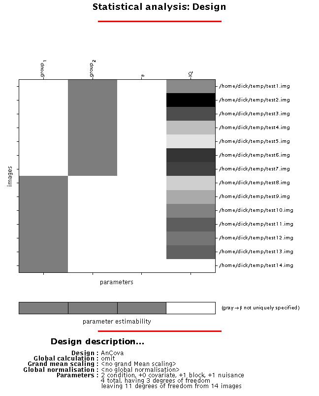
Display: SPM displays a design matrix having columns for each parameter (in this example, two groups, one constant (block), and one covariate (IQ in this example), and a row for each scan (subject). Again, the grey-and-white bar below the design matrix signals that the matrix is rank deficient (columns 1-3 are linearly dependent) which limits selection of meaningful contrasts (parameter weights) for group effects to those which sum up to zero (see 4).
File: the configuration for the design matrix will be saved as SPMcfg.mat in the working directory.
Finally, specify:
![]()
to begin parameter estimation now or at a later stage. If 'later', select 'Estimate' (middle panel) and select the appropriate SPMcfg.mat file.
N.B.
Model estimation may also be launched via the 'Explore design' option. SPM will prompt you to select a SPMcfg.mat file for inspection.
Clicking 'Design' (lower left window) will activate a pull-down menu which allows selection of displays for the design matrix, details of design orthogonality (surfable), selected scans and specified conditions, and covariates. It does not provide options to edit the model.
Output from Basic models parameter estimation (spm_spm.m):
beta_0001.img/hdr, ... : images containing parameter estimates for each column in the design matrix.
mask.hdr/img : mask image consisting of 0's and 1's indicating which voxels within the image volume are to be assessed.
ResMS.hdr/img : image of estimated residual variance.
RPV.hdr/img : image of estimated resels per voxel.
SPM.mat: contains details of design matrix, analysed images, search volume, smoothness estimates and results files.
xCon.mat: contains default F-contrast ('all effects' or 'effects of interest') which is used for selecting voxels at which to save raw data for future plotting.
Y.mad: contains (in compressed form) the raw (unsmoothed) data at voxels with an F-statistic higher than the default. Each column corresponds to one voxel, each row to an input image.
Yidx.mat: contains a 1 x N vector of column indices used in the Y.mad file (where N = number of available voxels).