4. Results assessment (spm_results_ui.m)
This section deals with the interactive exploration and characterisation of the results of a statistical analysis. For this purpose, three data sets will be discussed, which can be found at http://www.fil.ion.ucl.ac.uk/spm/data. These examples are (i) a single-subject epoch (block) fMRI study, (ii) a multi-subject PET study, (iii) a single-subject event-related fMRI study.
4.1 Example 1: single-subject fMRI block design (plotting and overlays)
This is a single-subject auditory activation study, with alternating 6-scan blocks of rest and binaural stimulation (speech). Details of model specification and parameter estimation can be found in the README_analysis.txt.
After completing model estimation (this is shown in the lower left SPM and Matlab windows), press 'Results'.
Select:
![]()
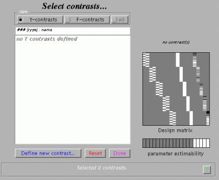
This will invoke the Contrast Manager:
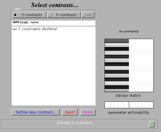
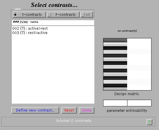
The contrast manager displays the design matrix (surfable) in the right panel and lists specified contrasts in the left panel. Either 't-contrast' or 'F-contrast' can be selected. One F-contrast is predefined ('effects of interest').
To examine statistical results for condition effects, select 'Define new contrast':
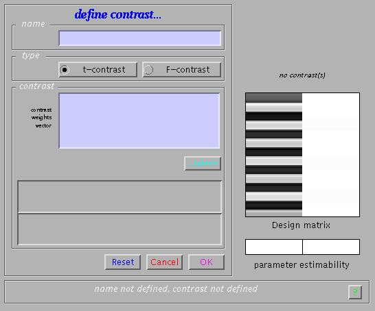
Main effects for the active condition (i.e., a one-sided t-test) can be specified (in this example) as '1' (active > rest) and '-1' (rest > active). SPM will accept correct contrasts only. Accepted contrasts are displayed at the bottom of the contrast manager window in green, incorrect ones are displayed in red. To view a contrast, select the contrast name (e.g., active>rest) and press 'Done':
Specify (no):
![]()
Masking implies selecting voxels specified by other contrasts. If 'yes', SPM will prompt for (one or more) masking contrasts, the significance level of the mask (default p = 0.05 uncorrected), and will ask whether an inclusive or exclusive mask should be used. Exclusive will remove all voxels which reach the default level of significance in the masking contrast, inclusive will remove all voxels which do not reach the default level of significance in the masking contrast. Masking does not affect p-values of the 'target' contrast, it only includes or excludes voxels.
Select (enter a title):
![]()
Specify (yes):
![]()
Select a height/amplitude threshold to examine results that are either corrected for multiple comparisons ('yes'), or uncorrected ('no') at a voxel-level.
Specify:
![]()
For corrected comparisons, the SPM default is p=0.05, for uncorrected comparisons, p=0.001.
Specify:
![]()
Select the number of voxels to restrict the minimum cluster size. 0 will include single voxel clusters ('spike' activations).
Output from Contrast Manager:
Files: images containing weighted parameter estimates are saved as con_0002.hdr/img, con_0003.hdr/img, ?etc. in the working directory. Images of T-statistics are saved as spmT_0002.hdr/img, spmT_0003.hdr/img.. etc., also in the working directory.
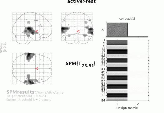
Display: in the Graphics window, SPM displays
a maximum intensity projection (MIP) on a glass brain in three orthogonal planes. The MIP is surfable: R-clicking in the MIP will activate a pulldown menu, L-clicking on the red cursor will allow it to be dragged to a new position.
the design matrix (showing the selected contrast). The design matrix is also surfable: R-clicking will show parameter names, L-clicking will show design matrix values for each scan.
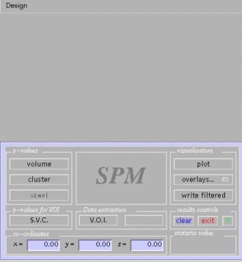
In the SPM Interactive window (lower left panel) a button box appears with various options for displaying statistical results (p-values panel) and creating plots/overlays (visualisation panel). Clicking 'Design' (upper left) will activate a pulldown menu as in the 'Explore design' option.
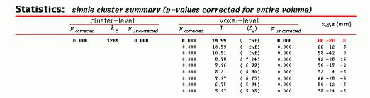
To get a summary of local maxima, press 'volume':
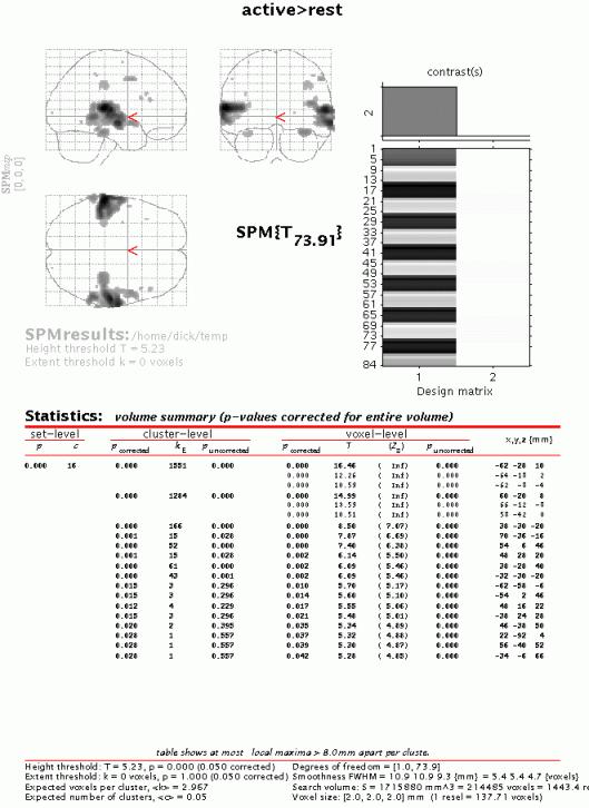
This will list all clusters above the chosen level of significance as well as separate (>8mm apart) maxima within a cluster, with details of significance thresholds and search volume underneath. The columns show, from right to left:
x, y, z (mm): coordinates in MNI space for each maximum where MNI space is an approximation to Talairach space.
voxel-level: the chance (p) of finding (under the null hypothesis) a voxel with this or a greater height (T- or Z-statistic), corrected / uncorrected for search volume
cluster-level: the chance (p) of finding a cluster with this or a greater size (ke), corrected / uncorrected for search volume
set-level: the chance (p) of finding this or a greater number of clusters (c) in the search volume
N.B.
The table is surfable: clicking a row of cluster coordinates will move the pointer in the MIP to that cluster, clicking other numbers will display the exact value in the Matlab window (e.g. 0.000 = 6.1971e-07).
To inspect a specific cluster (e.g., in this example data set, the R auditory cortex), either move the cursor in the MIP (by L-clicking & dragging the cursor, or R-clicking the MIP background which will activate a pulldown menu).
Alternatively, click the cluster coordinates in the volume table, or type the coordinates in the lower left windows of the SPM Interactive window.
Select 'cluster':
This will show coordinates and voxel-level statistics for local maxima (>4mm apart) in the selected cluster. This table is also surfable.
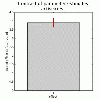
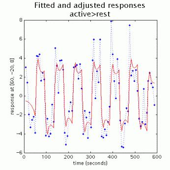
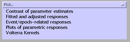
To plot effect size and/or signal time course from a voxel, e.g. for the cluster maximum, move the cursor to (60 -20 8). Next, press 'plot':
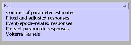
Contrast of parameter estimates: SPM will prompt for a specific contrast (e.g., active>rest). The plot will show effect size and error bars (in %).
Fitted and adjusted response: Plots adjusted data and fitted response across session/subject. SPM will prompt for a specific contrast and provides the option to choose different ordinates ('an explanatory variable', 'scan or time', or 'user specified'). If 'scan or time', the plot will show adjusted BOLD data (in %, blue dashed line) and the regressor(s) used (red solid line):
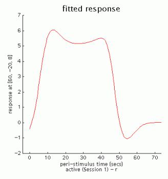
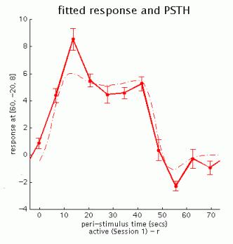
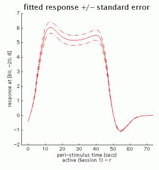
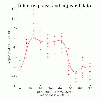
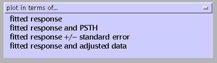
Event/epoch-related responses: Plots adjusted data and fitted response across peri-stimulus time. SPM provides four options:
fitted response: simple plot of mean (i.e., averaged over session) regressor(s) across PST
fitted response and PSTH (peri-stimulus time histogram): plots mean regressor(s) and mean signal +/- SE for each time bin.
fitted response +/- standard error: plots mean regressor(s) +/- SE
fitted response and adjusted data: plots regressor(s) and individual data (note that in this example the data are shown in columns due to the fixed TR/ISI relationship)
N.B.
The values for the fitted response across session/subject for the selected plot can be displayed and accessed in the Matlab window by typing 'Y'. Typing 'y' will display the adjusted data.
'Adjusted' data = adjusted for confounds (e.g., global flow) and high- and low pass filtering.
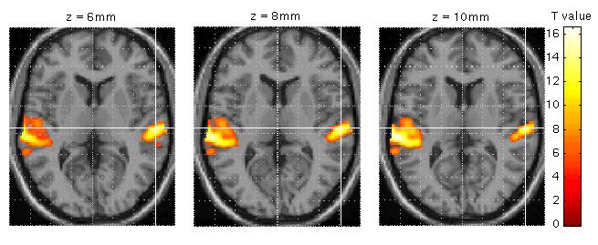
For anatomical visualisation of a cluster (in this example, R auditory cortex), press 'overlays' which will activate a pulldown menu. There are three options:
slices: overlay on three adjacent (2mm) transaxial slices. SPM will prompt for an image for rendering (a canonical image (see spm_template.man) or an individual T1/mean EPI image for single-subject analyses)
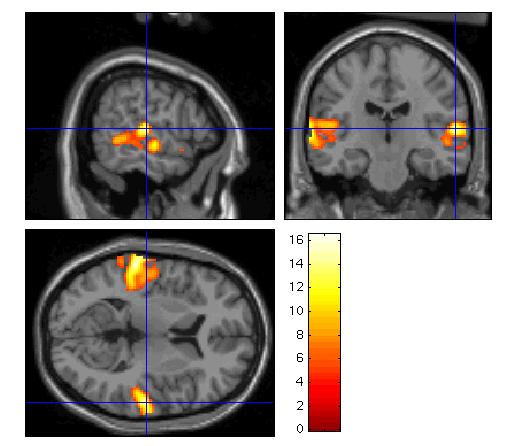
sections: overlay on three intersecting (sagittal, coronal, transaxial) slices. These renderings are surfable: clicking the images will move the crosshair
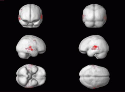
render: overlay on a volume rendered brain, with options for using a smoothed brain, and old (left) and new (right) style rendering.
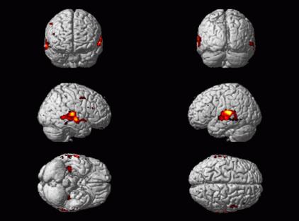
Renderings can be saved as filename.img and filename.hdr in the working directory by using the write filtered option.
Other options (in the results controls panel):
clear: clears lower subpanel of Graphics window
exit: exits the results section
? : launches spm_results_ui help
4.2 Example 2: Multi-subject PET study (volume of interest, masking and conjunction analyses)
This is a PET word generation study with five subjects, each having 12 scans, with alternating conditions of word shadowing (baseline) and word generation (active), randomised across subjects (see the README.txt). Although this data set can be analysed in several ways, it is suggested to select a subject-separable model (Multi-subj: cond x subj interaction & covariates, see 3.1). Specify: # covariates = 0, # nuisance variables = 0, GloNorm: AnCova by subject.
After completing model estimation (this is shown in the lower left SPM and Matlab windows), press 'Results'.
Select:
![]()
This will invoke the Contrast Manager:
To examine condition effects e.g. for subject 2, select 'Define new contrast'. Specify e.g. 'active>rest_subj2' (name) and '0 0 -1 1' (contrast), and press 'submit':
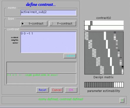
As shown, SPM will interpret '0 0 -1 1' as '0 0 -1 1 0 0 0 0 0 0'. Condition effects for each subject may be assessed as in the previous fMRI example.
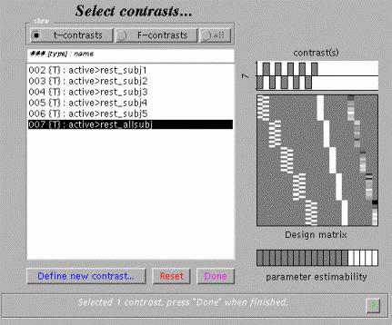
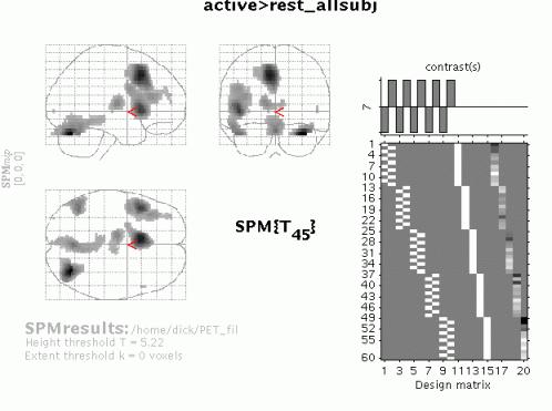
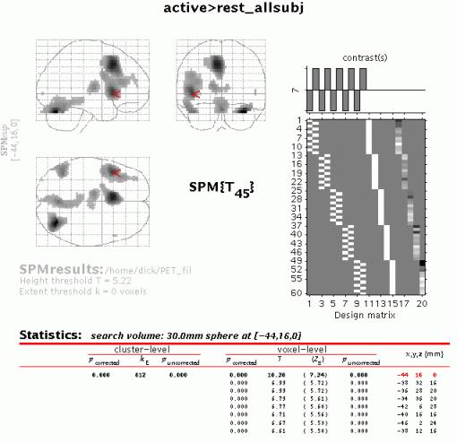
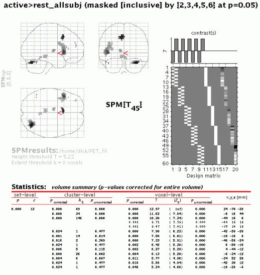
To examine group effects, define e.g. 'active>rest_allsubj' as '-1 1 -1 1 -1 1 -1 1 -1 1' and select it (press 'Done'):
Specify (no):
![]()
Masking implies selecting voxels specified by other contrasts. If 'yes', SPM will prompt for (one or more) masking contrasts, the significance level of the mask (default p = 0.05 uncorrected), and will ask whether an inclusive or exclusive mask should be used. Exclusive will remove all voxels which reach the default level of significance in the masking contrast, inclusive will remove all voxels which do not reach the default level of significance in the masking contrast. Masking does not affect p-values of the 'target' contrast.
Specify (yes):
![]()
Select a height/amplitude threshold to examine results that are either corrected for multiple comparisons ('yes'), or uncorrected ('no') at a voxel-level.
Specify:
![]()
For corrected comparisons, the SPM default is p=0.05, for uncorrected comparisons, p=0.001.
Specify:
![]()
Select the number of voxels to restrict the minimum cluster size. 0 will include single voxel clusters ('spike' activations).
Output from Contrast Manager:

Files: images containing weighted parameter estimates are saved as con_0002.hdr/img, con_0003.hdr/img, ?etc. in the working directory. Images of T-statistics are saved as spmT_0002.hdr/img, spmT_0003.hdr/img etc., also in the working directory.
Display: in the Graphics window, SPM displays
(i) a maximum intensity projection (MIP) on a glass brain in three orthogonal planes. The MIP is surfable: R-clicking in the MIP will activate a pulldown menu, L-clicking on the red cursor will allow it to be dragged to a new position.
the design matrix (showing the selected contrast). The design matrix is also surfable: R-clicking will show parameter names, L-clicking will show design matrix values for each scan.
In the SPM Interactive window (lower left panel) a button box appears with various options for displaying statistical results (p-values panel) and creating plots/overlays (visualisation panel). Clicking 'Design' (upper left) will activate a pulldown menu as in the 'Explore design' option.
To get a summary of local maxima, press 'volume':
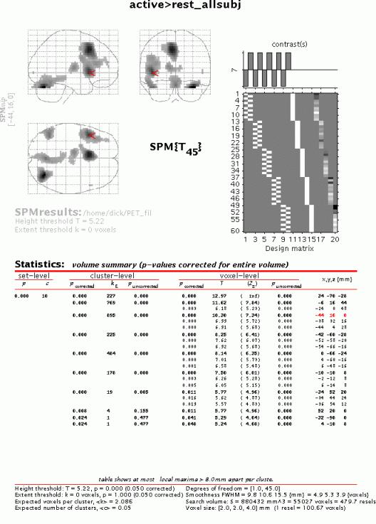
As in the previous example, this will list all clusters above the chosen level of significance as well as separate (>8mm apart) maxima within a cluster, with details of significance thresholds and search volume underneath. The columns show, from right to left:
x, y, z (mm): coordinates in MNI space for each maximum where MNI space is an approximation to Talairach space.
voxel-level: the chance (p) of finding (under the null hypothesis) a voxel with this or a greater height (T- or Z-statistic), corrected / uncorrected for search volume
cluster-level: the chance (p) of finding a cluster with this or a greater size (ke), corrected / uncorrected for search volume
set-level: the chance (p) of finding this or a greater number of clusters (c) in the search volume
N.B.
The table is surfable: clicking a row of cluster coordinates will move the pointer in the MIP to that cluster, clicking other numbers will display the exact value in the Matlab window (e.g. 0.000 = 6.1971e-07).
To inspect a specific cluster (e.g., in this example data set, the L prefrontal cortex), either move the cursor in the MIP (by L-clicking & dragging the cursor, or R-clicking the MIP background which will activate a pulldown menu).
Alternatively, click the cluster coordinates in the volume table, or type the coordinates in the lower left windows of the SPM Interactive window.
Select 'cluster':
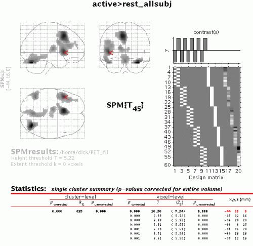
This will show coordinates and voxel-level statistics for local maxima (>4mm apart) in the selected cluster. The table is also surfable.
Both in the 'volume' and 'cluster' options, p-values are corrected for the entire search volume. If one has an a priori anatomical hypothesis (obviously, in the present example, that Broca's area will be activated during this word generation task) one may use the small volume correction option (see also Matthew Brett's tutorial at http://www.mrc-cbu.cam.ac.uk/Imaging/vol_corr.html). Select 'S.V.C.' (left lower panel), and select a suitable region, e.g., a 30mm sphere with its centre at -44 16 0. Note that the region should be defined using prior knowledge (e.g., a mask image derived from previous imaging data).
N.B.
As is shown, only corrected p-values change (become smaller) when SVC is used.
To extract a time course for data in this region of interest (spm.regions.m), select V.O.I. (Volume Of Interest) and select ('don't adjust'):
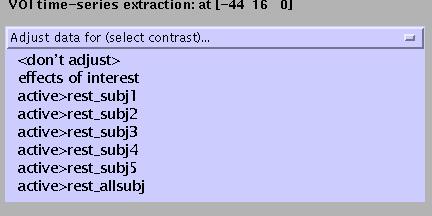
Specify (e.g., Broca):
![]()
Specify (accept default):
![]()
Output from spm.regions.m:
Display:
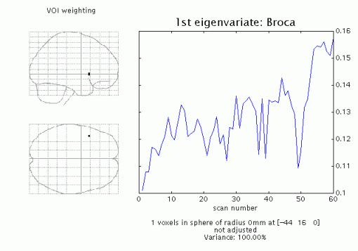
SPM displays a graph of the first eigenvariate of the data in or centered around the chosen voxel (or the nearest suprathreshold voxel saved in the Y.mad file), and lists the eigenvariate values (Y) in the Matlab window. If temporal filtering has been specified (fMRI), then the data is temporally filtered. Adjustment is with respect to the null space of a selected contrast, or can be omitted.
File: Y and VOI details (xY) are saved as VOI_regionname.mat in the working directory.
In this example, group effects are calculated averaged across subjects, therefore individual data may bias group results. To assess condition effects common to all subjects, one should either mask (inclusively) the 'all_subj' contrast with the individual contrasts, or perform a conjunction analysis.
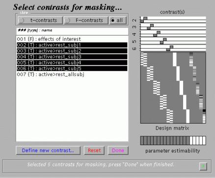
To assess the masked contrast, press 'Results', select the appropriate 'SPM.mat' file, and select the 'all_subj' contrast.
Next, press 'yes':
![]()
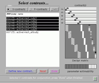
Select all individual contrasts (by pressing [control] while selecting):
Specify threshold (select default):
![]()
Select (inclusive):
![]()
Specify (accept default):
![]()
Specify (yes):
![]()
Specify (accept default):
![]()
Specify (accept default):
![]()
When the MIP appears, press 'volume':
The output shows all voxels which are (a) significant at p < 0.05 corrected across all subjects and (b) significant at p < 0.05 uncorrected for each subject individually.
To perform a conjunction across subjects, press 'Results', and select all individual contrasts (press 'Control'):
N.B.
Sometimes (e.g., if global confounds are used) the contrasts of parameter estimates are not exactly orthogonal (even if the contrast weight vectors are).
SPM checks whether the contrasts are orthogonal and if not makes them so (relative to the first contrast specified).
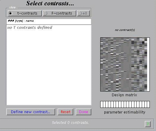
Next, press 'no':
![]()
Specify (accept):
Specify (yes):
![]()
Specify (accept default):
![]()
The p-value (corrected or uncorrected) refers to the threshold of the conjunction; SPM will compute corresponding thresholds for individual contrasts (for uncorrected thresholds, the individual threshold will be p1/n, where p = individual threshold and n = number of contrasts in the conjunction).
N.B.
In SPM99b, uncorrected p-values were applied by SPM to individual contrasts, so that the threshold of the conjunction was pn.
Height, and not extent, is used to specify thresholding because the distributional approximations for the spatial extent of a conjunction SPM are not known (at present), so that inference based on spatial extent is precluded.
When the MIP appears, press 'volume':
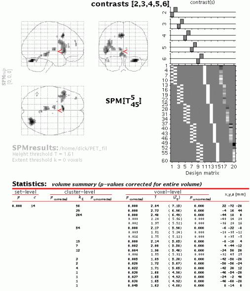
Although the MIP's of the masked group contrast and the conjunction are similar, for the conjunction an intersection SPM or 'minimum T-field' is computed. Conjunctions in SPM99 represent the intersection of several SPMs. This intersection is the same as thresholding a map of the minimum T-values (if the smallest T-value is above the specified threshold then all the T-values associated with the component SPMs are above threshold).
Conjunction SPMs are very useful for testing multiple hypotheses (each component hypothesis being specified by a contrast). In this example, the set of hypotheses tested jointly is that the first subject did not activate, the second subject did not activate and so on. In regions that survive a conjunction analysis the null hypothesis is rejected jointly for all subjects. This can be thought of as enabling an inference that subject 1 activated AND subject 2 activated AND subject 3... etc.
Gaussian field theory results are available for SPMs of minimum T- (or F-) statistics and therefore corrected p-values can be computed. Note that the minimum T-values do not have the usual Student's T-distribution and small minimum T-values can be very significant.
Example 3: single-subject fMRI event-related design (F-contrasts)
As a third and more sophisticated example, consider the data from a repetition priming experiment performed using event-related fMRI. Again, details regarding the data set can be found in the README.txt. Briefly, this is a 2x2 factorial study where famous and non-famous faces were presented twice (while the subject was asked to make fame judgements) against a checkerboard baseline. There are thus four event-types of interest, (first and second presentations of famous and non-famous faces, ordered in the design matrix N1-N2-F1-F2), each modelled with a canonical HRF and its temporal derivative. Also included are two event-types of no interest - the (rare) errors made by this subject on the fame-judgement task - and the subject's realignment parameters, to regress out residual movement-related variance. The latter can be achieved by loading the realignment_*.txt file (output from the realignment stage) as a matrix into the Matlab workspace and entering the matrix name in the SPM input box (rather than specifying 6 vectors of length 351 in this example). Preprocessing of the data includes slice timing correction having the middle slice (12) as the reference slice. Therefore, prior to specifying the model, in the fMRI statistics defaults, the sampled bin should be equal to half the number of bins. For example, enter number of bins = 24 (the number of slices) and the sampled bin=12, using the Defaults button. In addition, stimulus onset times have been specified as a cell array variable, allowing different vector (row) lengths for separate trials.
In addition to analysing the data in the above "categorical" design, an alternative "parametric" design is illustrated in which repetition is viewed as a continuum. In this case, the response to each presentation of famous and non-famous faces is modulated by the time interval (lag) since the previous presentation of that face (for first presentations, this lag is infinite).
To assess the results for the categorical (factorial) analysis, specify and estimate the model (alternatively download the CatStats files). Next, press 'Results' and select the appropriate SPM.mat file. This will again invoke the contrast manager:
To assess the main effects of viewing faces vs. baseline, select 'Define new contrast' and type 'Canonical HRF: Faces > Baseline' (name) and '1 0 1 0 1 0 1 0' (contrast), and press 'Done'.
Specify (no):
![]()
Specify (accept default):
![]()
After computation of the contrast, specify (yes):
![]()
Specify (accept default):
![]()
Specify (accept default):
![]()
When the MIP appears, press 'volume':
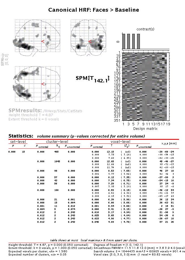
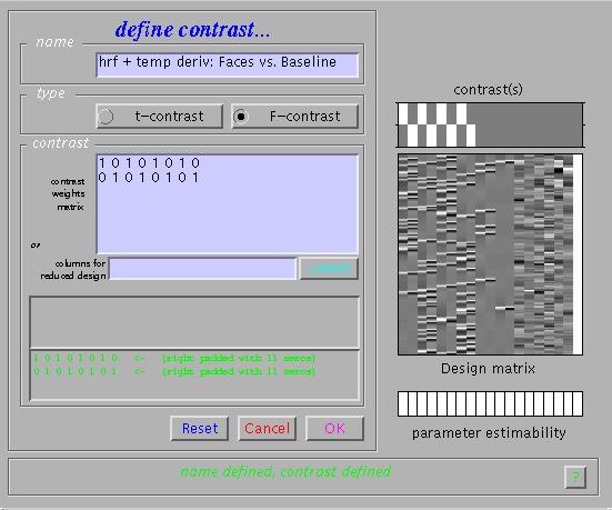
The table lists all areas where the mean of the parameter estimates for the canonical hrf of the four conditions is significantly greater than baseline (zero). To assess both the hrf and its temporal derivative, an F-contrast is required. Press 'Results', select the SPM.mat file, and press 'F-contrast' (radio button). Next, select 'Define new contrast', specify 'hrf + temp deriv: Faces vs. Baseline' (name) and enter
'1 0 1 0 1 0 1 0
0 1 0 1 0 1 0 1 ' (contrast) and press 'Done':
Select the new contrast, specify 'mask with other images?' (no), specify 'name of comparison' (accept default), specify 'corrected height threshold' (yes), specify 'corrected p value' (accept default). Again, when the MIP appears, press 'volume':
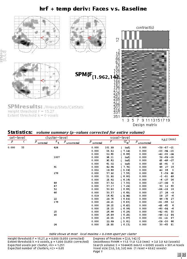
Although the MIP of this F-contrast looks similar to the previous t-contrast, note that the present contrast shows the areas for which the mean of the parameter estimates for the canonical hrf OR its temporal derivative for the four conditions are different from zero (baseline). In other words, the F-contrast is two-sided, and tests two t-contrasts simultaneously. Also note that an F- (or t-) contrast such as 1 1 1 1 1 1 1 1, which tests whether the mean of the canonical hrf AND its temporal derivative for all conditions are different from (larger than) zero is not sensible. This is because the canonical hrf and its temporal derivative may cancel each other out while being significant in their own right. Finally, note that single F-contrasts can be regarded as t-contrasts^2, so that the F-contrasts 1 0 -1 0 1 0 -1 0 and -1 0 1 0 -1 0 1 0 are equivalent.
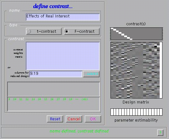
The relative contributions of the canonical hrf and its temporal derivative at a given voxel may also be assessed using F-contrasts to estimate a reduced model, removing all confounds. Press 'Results', select the SPM.mat file, press 'F-contrast' in the contrast manager, and select 'Define new contrast'. Specify 'Effects of Real Interest' (name) and type '9:19' in the small window labelled 'columns for reduced design'. This will remove columns 9 to 19 (i.e., hrf and temporal derivative for events representing error judgements and nuisance covariates) from the design.
Submit and select the new contrast, specify 'mask with other images?' (no), specify 'name of comparison' (accept default), specify 'corrected height threshold' (yes), specify 'corrected p value' (accept default). Again, when the MIP appears, press 'volume':
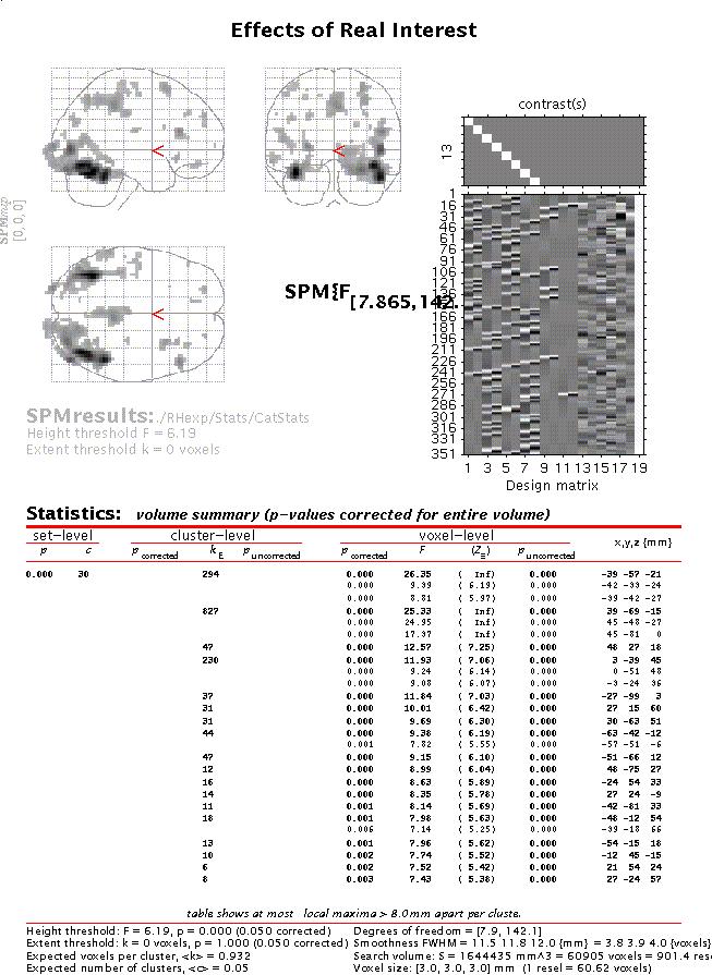
Move the cursor to e.g. the anterior right fusiform blob (the R fusiform face area) by clicking the second set of coordinates in the cluster (45 -48 -27) and press 'plot'. Select 'Contrast of parameter estimates' and select 'Effects of real interest':
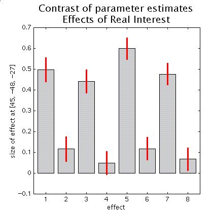
Columns 1,3,5,7 are the canonical hrfs for N1 (non-famous faces, first presentation), N2 (non-famous faces, second presentation), F1 (famous faces, 1st presentation) and F2 (famous faces, 2nd presentation), whereas columns 2,4,6,8 are the temporal derivatives. Note that the amplitude of the canonical hrfs is large compared to the temporal derivatives, suggesting that, for this region at least, the timing of the model is adequate. Also note the repetition x stimulus type interaction (the decrease from N1 to N2 is smaller than for F1 to F2).
To assess further the effects of stimulus repetition, press 'Results', select the SPM.mat file, and press 'F-contrast'. Specify e.g. 'hrf + temp deriv: 1 vs. 2' (name) and
'1 0 -1 0 1 0 -1 0
0 1 0 -1 0 1 0 -1' (contrast). Submit and select the contrast. Specify 'mask with another contrast' (yes), select the 'Canonical HRF: Faces > Baseline' t-contrast, specify 'threshold for mask' (accept default of p=0.05 uncorrected), specify 'nature of mask' (inclusive), specify 'title for comparison' (accept default), specify 'corrected height threshold' (no), specify threshold (0.001).
Again, when the MIP appears, press 'volume':
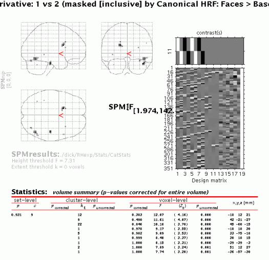
The MIP shows all clusters where the difference between the parameter estimates for first and second presentations for the canonical hrf OR its temporal derivative is significantly different from zero AND the canonical hrf for all four conditions is significantly larger than zero. Note that although the mask does not alter the threshold for the target contrast, the combined probability for a voxel to appear in the masked contrast is in the order of 0.05 x 0.001 uncorrected due to the orthogonality of the contrasts.
To plot repetition suppression effects for the R fusiform region, select the third cluster from the top (by clicking 48 60 -15; slightly more posterior to that identified above) and press 'plot'.
Select 'event/epoch-related responses':
Specify '1:4':
![]()
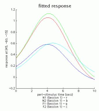
Select 'fitted response':
To adjust the scale of the x-axis (time), press 'attrib' from the plot controls panel:
Select Xlim, and change the default (-4 32) to '0 10':
![]()
Note the signal decrease between first and second presentations of both famous and non-famous faces:
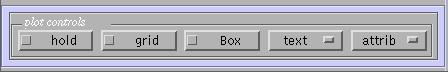
Other options from the plot controls panel:
hold: allows overlaying of plots
grid: toggles between grid on/off
Box: toggles between axes/box
text: allows editing of title and/or axis labels.
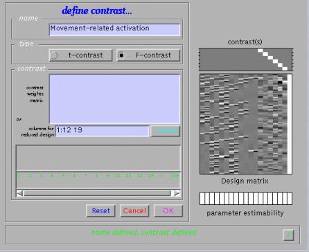
To assess movement-related activation, press 'Results', select the SPM.mat file, and select 'F-contrast' in the Contrast Manager. Specify e.g. 'Movement-related activation' (name) and either
'0 0 0 0 0 0 0 0 0 0 0 0 1
0 0 0 0 0 0 0 0 0 0 0 0 0 1
0 0 0 0 0 0 0 0 0 0 0 0 0 0 1
0 0 0 0 0 0 0 0 0 0 0 0 0 0 0 1
0 0 0 0 0 0 0 0 0 0 0 0 0 0 0 0 1
0 0 0 0 0 0 0 0 0 0 0 0 0 0 0 0 0 1'
in the 'contrasts weights matrix' window, or '1:12 19' in the 'columns for reduced design' window.
Submit and select the contrast, specify 'mask with other contrasts?' (no), 'title for comparison' (accept default), 'corrected height threshold' (yes), and 'corrected p-value' (accept default). When the MIP appears, press 'volume':
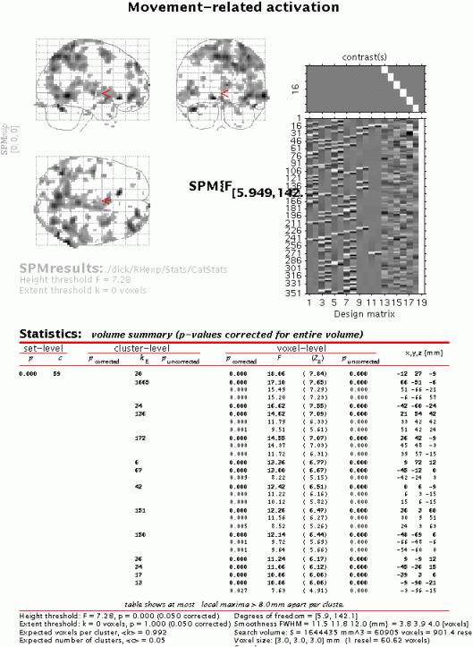
The table displays all clusters where signal changes correlated with any of the six movement parameters are significantly different from zero. Note the large edge effects, which, however, are not apparent in the fusiform regions.
Finally, consider the effects of the interval between first and second presentations of famous and non-famous faces. For this purpose, an alternative statistical model needs to be estimated, with four trial types. (1) First and second presentation of a non-famous face (N1 and N2 collapsed). (2) First and second presentation of a famous face (F1 and F2 collapsed). (3) Errors in judging non-famous faces. (4) Errors in judging famous faces. These are modelled with the canonical hrf alone, with two parametric (exponential) modulations added for second presentations of non-famous and famous faces. See the README.txt for details of design specification.
After completion of model estimation, press 'Results' and select the SPM.mat file. When the Contrast Manager appears, define an F-contrast 'Effect of Lag (on canonical N+F)' (name) and '0 1 0 1', and a t-contrast 'Canonical: Faces>Baseline' (name) and '1 0 1 0'. Select the F-contrast, specify 'mask with other contrasts' (yes), select 'Canonical: Faces>Baseline', specify 'uncorrected mask p-value' (accept default), 'nature of mask (inclusive), 'title for comparison' (accept default), 'corrected height threshold' (no), and 'corrected p-value' (accept default). When the MIP appears, press 'volume':
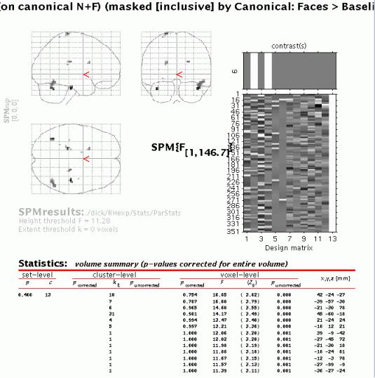
The table displays all clusters where the exponential change in activation between first and second presentations for famous OR non-famous faces for the canonical hrf is significantly different from zero AND the canonical hrf for the first two conditions is significantly larger than zero (baseline). To plot these parametric effects, select the R fusiform region (45 -60 -18, similar to the region identified in the previous categorical analysis for repetition effects), and press 'plot'. Select 'Plots of parametric responses' and select 'F' (or 'N'). Note that the 'attrib' option does not allow adjustment of the scale of the Z-axis; therefore, to change the scale for all axes, type e.g. 'figure (1), axis ([0 30 0 100 0 1])' in the Matlab window.
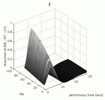
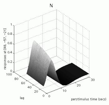
Note that these repetition effects are transient (decrease with increasing intervals between first and second presentations), especially for famous faces.