No Pre-processing

Use ECMOCO

1. Target image: Because this toolbox uses the optimization function of spm_coreg, it is modality independent, i.e. in theory any low-b-value image or high-b-value image can be used as target – provided the SNR of the DTI dataset is high enough. Recommended is using the low-b-value image, because it suffers less from EC-related image distortions.

2. Source images: Select all images of the DTI dataset that are supposed to be corrected for drift, motion and EC image distortions.

3. Choose the parameters, which you want to correct. You can choose between 12 affine parameters. The 4 eddy current parameters are displayed in Figure 1. We propose three sets of parameters for different purposes (see below), but you can select the parameters freely.

Proposed parameters:

a) Correcting only for subject motion: [1 1 1 1 1 1 0 0 0 0 0 0];

b) Correcting only for subject motion and whole-brain eddy currents:

[1 1 1 1 1 1 0 1 0 1 1 0];

c) Correcting distortions in a spherical phantom: [1 1 1 0 0 0 1 0 1 1 0]. Note that the input vector for this parameter must have 12 binary components, i.e. for each component you can choose between 0 and 1 (0: the parameter is not estimated; 1: the parameter is estimated).

4. Choose whether you want to write the registered images. By default the write images option is on. For each image a matfile is written, which contains the registration parameters (starting with prefix: “mut”).

5. Choose whether you want to see the estimated EC and motion parameters for each image. This option might be helpful to provide you with a feeling about the artefact level in your dataset (see Fig. 2). You might want to turn it off if more than one subject is registered, because two figures will be displayed for each subject. Note that those figures will also be written in “eps”-format.

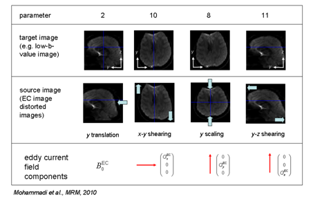
Fig. 1: The whole-brain eddy current distortions (3^rd row) are corrected by affine transformations when the corresponding parameters (2, 8, 10 and 11, 1^st row) are enabled. Note that this toolbox only corrects for image distortions that are related to the linear components of the EC field (4^th row).

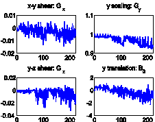
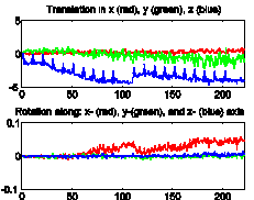
Fig. 2: The EC (left) and motion (right) parameters for an example DTI dataset with more than 200 images.

Referencing

Please cite the following paper when using this toolbox:

Mohammadi S, Moller HE, Kugel H, Muller DK, Deppe M (2010) Correcting eddy current and motion effects by affine whole-brain registrations: evaluation of three-dimensional distortions and comparison with slicewise correction. Magn Reson Med 64: 1047-1056; doi: 10.1002/mrm.22501.