1. Introduction

2. Functional specialization and integration

3. Spatial realignment and normalisation

4. Statistical Parametric Mapping

5. Experimental design

6. Designing fMRI studies

7. Inferences about subjects and populations

8. Effective Connectivity

9. References

6. Designing fMRI studies

In this section we consider fMRI time-series from a signal processing perspective with particular reference to optimal experimental design and efficiency. fMRI time-series can be viewed as a linear admixture of signal and noise. Signal corresponds to neuronally mediated hemodynamic changes that can be modeled as a [non]linear convolution of some underlying neuronal process, responding to changes in experimental factors, by a HRF. Noise has many contributions that render it rather complicated in relation to other neurophysiological measurements. These include neuronal and non-neuronal sources. Neuronal noise refers to neurogenic signal not modeled by the explanatory variables and has the same frequency structure as the signal itself. Non-neuronal components have both white [e.g. R.F. (Johnson) noise] and colored components [e.g. pulsatile motion of the brain caused by cardiac cycles and local modulation of the static magnetic field B₀ by respiratory movement]. These effects are typically low frequency or wide-band (e.g. aliased cardiac-locked pulsatile motion). The superposition of all these components induces temporal correlations among the error terms (denoted by in Figure 3) that can effect sensitivity to experimental effects. Sensitivity depends upon (i) the relative amounts of signal and noise and (ii) the efficiency of the experimental design. Efficiency is simply a measure of how reliable the parameter estimates are and can be defined as the inverse of the variance of a contrast of parameter estimates (see Figure 3). There are two important considerations that arise from this perspective on fMRI time-series: The first pertains to optimal experimental design and the second to optimum [de]convolution of the time-series to obtain the most efficient parameter estimates.

6.1 The hemodynamic response function and optimum design

As noted above, a LTI model of neuronally mediated signals in fMRI suggests that, whatever the frequency structure of experimental variables, only those that survive convolution with the hemodynamic response function (HRF) can be estimated with any efficiency. By convolution theorem the experimental variance should therefore be designed to match the transfer function of the HRF. The corresponding frequency profile of this transfer function is shown in Figure 9 - solid line). It is clear that frequencies around 0.03 Hz are optimal, corresponding to periodic designs with 32 second periods (i.e. 16 second epochs). Generally, the first objective of experimental design is to comply with the natural constraints imposed by the HRF and ensure that experimental variance occupies these intermediate frequencies.

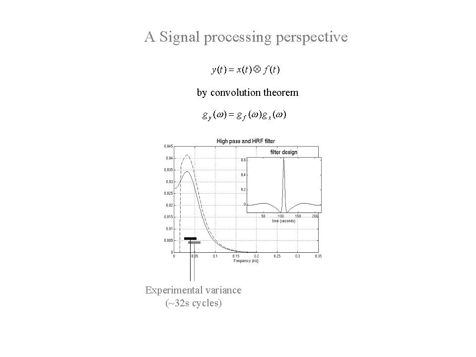
Figure 9. Modulation transfer function of a canonical hemodynamic response function (HRF), with (broken line) and without (solid line) the addition of a high pass filter. This transfer function corresponds to the spectral density of a white noise process after convolution with the HRF and places constraints on the frequencies that are survive convolution with the HRF. This follows from convolution theorem (summarized in the equations). The insert is the filter expressed in time, corresponding to the spectral density that obtains after convolution with the HRF and high-pass filtering.

6.2 Serial correlations and filtering

This is quite a complicated but important area. Conventional signal processing approaches dictate that whitening the data engenders the most efficient parameter estimation. This corresponds to filtering with a convolution matrix S (see Figure 3) that is the inverse of the intrinsic convolution matrix K (). This whitening strategy renders the generalized least squares estimator in Figure 3 equivalent to the Gauss-Markov estimator or minimum variance estimator. However, one generally does not know the form of the intrinsic correlations, which mean it has to be estimated. This estimation usually proceeds using a restricted maximum likelihood (ReML) estimate of the serial correlations, among the residuals, that properly accommodates the effects of the residual-forming matrix and associated loss of degrees of freedom. However, using this estimate of the intrinsic non-sphericity to form a Gauss-Markov estimator at each voxel has several problems. (i) First the estimate of non-sphericity can itself be very inefficient leading to bias in the standard error (Friston et al 2000b). (ii) ReML estimation requires an iterative procedure at every voxel and this is computationally prohibitive. (iii) Adopting a different form for the serial correlations at each voxel means the effective degrees of freedom and the null distribution of the statistic will change from voxel to voxel. This violates the assumptions of GRF results for T and F fields (although not very seriously). There are a number of different approaches to these problems that aim to increase the efficiency of the estimation and reduce the computational burden. The approach we have chosen is to forgo the efficiency of the Gauss-Markov estimator and use a generalized least square GLS estimator, after approximately whitening the data with a high-pass filter. The GLS estimator is unbiased and, luckily, is identical to the Gauss-Markov estimator if the regressors in the design matrix are periodic². After GLS estimation is estimated using ReML and the resulting estimate of entered into the expression for the standard error and degrees of freedom provided in Figure 3. To ensure this non-sphericity estimate is robust, we assume it is the same at all voxels. Clearly this is an approximation but can be motivated by the fact we have applied the same high-pass temporal convolution matrix S to all voxels. This ameliorates any voxel to voxel variations in (see Figure 3)

The reason that high-pass filtering approximates a whitening filter is that there is a preponderance of low frequencies in the noise. fMRI noise has been variously characterized as a 1/f process (Zarahn et al 1997) or an autoregressive process (Bullmore et al 1996) with white noise (Purdon and Weisskoff 1998). Irrespective of the exact form these serial correlations take, high-pass filtering suppresses low frequency components in the same way that whitening would. An example of a band-pass filter with a high-pass cut-off of 1/64 Hz is shown in inset of Figure 7. This filter's transfer function (the broken line in the main panel) illustrates the frequency structure of neurogenic signals after high-pass filtering.

6.3 Spatially coherent confounds and global normalization

Implicit in the use of high pass filtering is the removal of low frequency components that can be regarded as confounds. Other important confounds are signal components that are artifactual or have no regional specificity. These are referred to as global confounds and have a number of causes. These can be divided into physiological (e.g. global perfusion changes in PET, mediated by changes in pCO₂) and non-physiological (e.g. transmitter power calibration, B₁ coil profile and receiver gain in fMRI). The latter generally scale the signal before the MRI sampling process. Other non-physiological effects may have a non-scaling effect (e.g. Nyquist ghosting, movement-related effects etc). In PET it is generally accepted that regional changes in rCBF, evoked neuronally, mix additively with global changes to give the measured signal. This calls for a global normalization procedure where the global estimator enters into the statistical model as a confound. In fMRI, instrumentation effects that scale the data motivate a global normalization by proportional scaling, using the whole brain mean, before the data enter into the statistical model.

It is important to differentiate between global confounds and their estimators. By definition the global mean over intra-cranial voxels will subsume regionally specific effects. This means that the global estimator may be partially collinear with effects of interest, especially if the evoked responses are substantial and widespread. In these situations global normalization may induce apparent deactivations in regions not expressing a physiological response. These are not artifacts in the sense they are real, relative to global changes, but they have little face validity in terms of the underlying neurophysiology. In instances where regionally specific effects bias the global estimator, some investigators prefer to omit global normalization. Provided drift terms are removed from the time-series, this is generally acceptable because most global effects have slow time constants. However, the issue of normalization-induced deactivations is better circumnavigated with experimental designs that use well-controlled conditions, which elicit differential responses in restricted brain systems.

6.4 Nonlinear system identification approaches

So far we have only considered LTI models and first order HRFs. Another signal processing perspective is provided by nonlinear system identification (Vazquez and Noll 1998). This section considers nonlinear models as a prelude to the next subsection on event-related fMRI, where nonlinear interactions among evoked responses provide constraints for experimental design and analysis. We have described an approach to characterizing evoked hemodynamic responses in fMRI based on nonlinear system identification, in particular the use of Volterra series (Friston et al 1998a). This approach enables one to estimate Volterra kernels that describe the relationship between stimulus presentation and the hemodynamic responses that ensue. Volterra series are essentially high order extensions of linear convolution models. These kernels therefore represent a nonlinear characterization of the HRF that can model the responses to stimuli in different contexts and interactions among stimuli. In fMRI, the kernel coefficients can be estimated by (i) using a second order approximation to the Volterra series to formulate the problem in terms of a general linear model and (ii) expanding the kernels in terms of temporal basis functions. This allows the use of the standard techniques described above to estimate the kernels and to make inferences about their significance on a voxel-specific basis using SPMs.

One important manifestation of the nonlinear effects, captured by the second order kernels, is a modulation of stimulus-specific responses by preceding stimuli that are proximate in time. This means that responses at high stimulus presentation rates saturate and, in some instances, show an inverted U behavior. This behavior appears to be specific to BOLD effects (as distinct from evoked changes in cerebral blood flow) and may represent a hemodynamic refractoriness. This effect has important implications for event-related fMRI, where one may want to present trials in quick succession (see below).

The results of a typical nonlinear analysis are given in Figure 10. The results in the right panel represent the average response, integrated over a 32-second train of stimuli as a function of stimulus onset asynchrony (SOA) within that train. These responses were based on the kernel estimates (left hand panels) using data from a voxel in the left posterior temporal region of a subject obtained during the presentation of single words at different rates. The solid line represents the estimated response and shows a clear maximum at just less than one second. The dots are responses based on empirical data from the same experiment. The broken line shows the expected response in the absence of nonlinear effects (i.e. that predicted by setting the second order kernel to zero). It is clear that nonlinearities become important at around two seconds leading to an actual diminution of the integrated response at sub-second SOAs. The implication of this sort of result is that (i) SOAs should not really fall much below one second and (ii) at short SOAs the assumptions of linearity are violated. It should be noted that these data pertain to single word processing in auditory association cortex. More linear behaviors may be expressed in primary sensory cortex where the feasibility of using minimum SOAs as low as 500ms has been demonstrated (Burock et al 1998). This lower bound on SOA is important because some effects are detected more efficiently with high presentation rates. We now consider this from the point of view of and event-related designs.

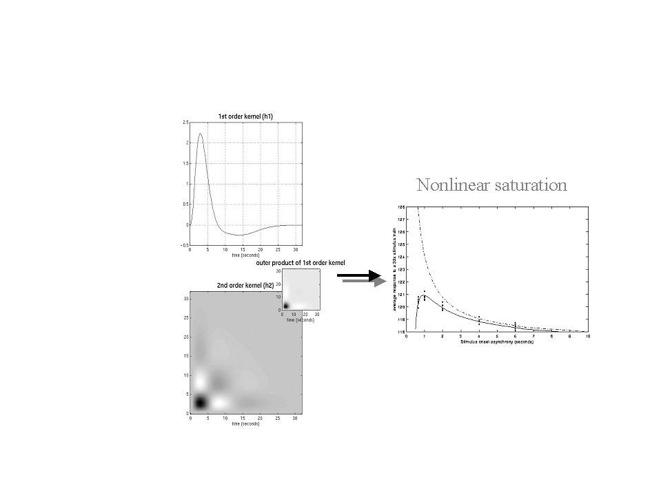
Figure 10. Left panels: Volterra kernels from a voxel in the left superior temporal gyrus at -56, -28, 12mm. These kernel estimates were based on a single subject study of aural word presentation at different rates (from 0 to 90 words per minute) using a second order approximation to a Volterra series expansion modeling the observed hemodynamic response to stimulus input (a delta function for each word). These kernels can be thought of as a characterization of the second order hemodynamic response function. The first order kernel (upper panel) represents the (first order) component usually presented in linear analyses. The second order kernel (lower panel) is presented in image format. The color scale is arbitrary; white is positive and black is negative. The insert on the right represents the second order kernel that would be predicted by a simple model that involved linear convolution with followed by some static nonlinearly.

Right panel: Integrated responses over a 32-second stimulus train as a function of SOA. Solid line: Estimates based on the nonlinear convolution model parameterized by the kernels on the left. Broken line: The responses expected in the absence of second order effects (i.e. in a truly linear system). Dots: Empirical averages based on the presentation of actual stimulus trains.

6.5 Event and epoch-related designs

A crucial distinction, in experimental design for fMRI, is that between epoch and event-related designs. In SPECT and PET only epoch-related responses can be assessed because of the relatively long half-life of the radiotracers used. However, in fMRI there is an opportunity to measure event-related responses that may be important in some cognitive and clinical contexts. An important issue, in event-related fMRI, is the choice of inter-stimulus interval or more precisely SOA. The SOA, or the distribution of SOAs, is a critical factor in experimental design and is chosen, subject to psychological or psychophysical constraints, to maximize the efficiency of response estimation. The constraints on the SOA clearly depend upon the nature of the experiment but are generally satisfied when the SOA is small and derives from a random distribution. Rapid presentation rates allow for the maintenance of a particular cognitive or attentional set, decrease the latitude that the subject has for engaging alternative strategies, or incidental processing, and allows the integration of event-related paradigms using fMRI and electrophysiology. Random SOAs ensure that preparatory or anticipatory factors do not confound event-related responses and ensure a uniform context in which events are presented. These constraints speak to the well-documented advantages of event-related fMRI over conventional blocked designs (Buckner et al 1996, Clark et al 1998).

In order to compare the efficiency of different designs it is useful to have some common framework that accommodates them all. The efficiency can then be examined in relation to the parameters of the designs. Designs can be stochastic or deterministic depending on whether there is a random element to their specification. In stochastic designs (Heid et al 1997) one needs to specify the probabilities of an event occurring at all times those events could occur. In deterministic designs the occurrence probability is unity and the design is completely specified by the times of stimulus presentation or trials. The distinction between stochastic and deterministic designs pertains to how a particular realization or stimulus sequence is created. The efficiency afforded by a particular event sequence is a function of the event sequence itself, and not of the process generating the sequence (i.e. deterministic or stochastic). However, within stochastic designs, the design matrix X, and associated efficiency, are random variables and the expected or average efficiency, over realizations of X is easily computed.:

In the framework considered here (Friston et al 1999a) the occurrence probability p of any event occurring is specified at each time that it could occur (i.e. every SOA). Here p is a vector with an element for every SOA. This formulation engenders the distinction between stationary stochastic designs, where the occurrence probabilities are constant and non-stationary stochastic designs, where they change over time. For deterministic designs the elements of p are 0 or 1, the presence of a 1 denoting the occurrence of an event. An example of p might be the boxcars used in conventional block designs. Stochastic designs correspond to a vector of identical values and are therefore stationary in nature. Stochastic designs with temporal modulation of occurrence probability have time-dependent probabilities varying between 0 and 1. With these probabilities the expected design matrices and expected efficiencies can be computed. A useful thing about this formulation is that by setting the mean of the probabilities p to a constant, one can compare different deterministic and stochastic designs given the same number of events. Some common examples are given in Figure 11 (right panel) for an SOA of 1 second and 32 expected events or trials over a 64 second period (except for the first deterministic example with 4 events and an SOA of 16 seconds). It can be seen that the least efficient is the sparse deterministic design (despite the fact that the SOA is roughly optimal for this class), whereas the most efficient is a block design. A slow modulation of occurrence probabilities gives high efficiency whilst retaining the advantages of stochastic designs and may represent a useful compromise between the high efficiency of block designs and the psychological benefits and latitude afforded by stochastic designs. However, it is important not to generalize these conclusions too far. An efficient design for one effect may not be the optimum for another, even within the same experiment. This can be illustrated by comparing the efficiency with which evoked responses are detected and the efficiency of detecting the difference in evoked responses elicited by two sorts of trials:

Consider a stationary stochastic design with two trial types. Because the design is stationary the vector of occurrence probabilities, for each trial type, is specified by a single probability. Let us assume that the two trial types occur with the same probability p. .By varying p and SOA one can find the most efficient design depending upon whether one is looking for evoked responses per se or differences among evoked responses. These two situations are depicted in the left panels of Figure 11. It is immediately apparent that, for both sorts of effects, very small SOAs are optimal. However, the optimal occurrence probabilities are not the same. More infrequent events (corresponding to a smaller p = 1/3) are required to estimate the responses themselves efficiently. This is equivalent to treating the baseline or control condition as any other condition (i.e. by including null events, with equal probability, as further event types). Conversely, if we are only interested in making inferences about the differences, one of the events plays the role of a null event and the most efficient design ensues when one or the other event occurs (i.e. p = 1/2). In short, the most efficient designs obtain when the events subtending the differences of interest occur with equal probability.

Another example, of how the efficiency is sensitive to the effect of interest, is apparent when we consider different parameterizations of the HRF. This issue is sometimes addressed through distinguishing between the efficiency of response detection and response estimation. However, the principles are identical and the distinction reduces to how many parameters one uses to model the HRF for each trail type (one basis function is used for detection and a number are required to estimate the shape of the HRF). Here the contrasts may be the same but the shape of the regressors will change depending on the temporal basis set employed. The conclusions above were based on a single canonical HRF. Had we used a more refined parameterization of the HRF, say using three-basis functions, the most efficient design to estimate one basis function coefficient would not be the most efficient for another. This is most easily seen from the signal processing perspective where basis functions with high frequency structure (e.g. temporal derivatives) require the experimental variance to contain high frequency components. For these basis functions a randomized stochastic design may be more efficient than a deterministic block design, simply because the former embodies higher frequencies. In the limiting case of FIR estimation the regressors become a series of stick functions (see Figure 5) all of which have high frequencies. This parameterization of the HRF calls for high frequencies in the experimental variance. However, the use of FIR models is contraindicated by model selection procedures (Henson et al in preparation) that suggest only two or three HRF parameters can be estimated with any efficiency. Results that are reported in terms of FIRs should be treated with caution because the inferences about evoked responses are seldom based on the FIR parameter estimates. This is precisely because they are estimated inefficiently and contain little useful information.

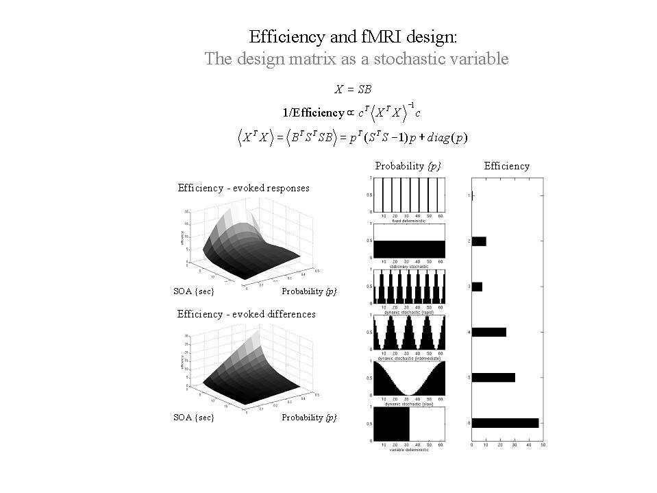
Figure 11. Efficiency as a function of occurrence probabilities p. for a model X formed by post-multiplying S (a matrix containing n columns, modeling n possible event-related responses every SOA) by B. B is a random binary vector that determines whether the nth response is included in X or not, where . Right panels: A comparison of some common designs. A graphical representation of the occurrence probabilities p expressed as a function of time (seconds) is shown on the left and the corresponding efficiency is shown on the right. These results assume a minimum SOA of one second, a time-series of 64 seconds and a single trial-type. The expected number of events was 32 in all cases (apart from the first). Left panels: Efficiency in a stationary stochastic design with two event types both presented with probability p every SOA. The upper graph is for a contrast testing for the response evoked by one trial type and the lower graph is for a contrast testing for differential responses.