1. Introduction

2. Functional specialization and integration

3. Spatial realignment and normalisation

4. Statistical Parametric Mapping

5. Experimental design

6. Designing fMRI studies

7. Inferences about subjects and populations

8. Effective Connectivity

9. References

3. Spatial realignment and normalisation

The analysis of neuroimaging data generally starts with a series of spatial transformations. These transformations aim to reduce artifactual variance components in the voxel time-series that are induced by movement or shape differences among a series of scans. Voxel-based analyses assume that the data from a particular voxel all derive from the same part of the brain. Violations of this assumption will introduce artifactual changes in the voxel values that may obscure changes, or differences, of interest.. Even single-subject analyses proceed in a standard anatomical space, simply to enable reporting of regionally-specific effects in a frame of reference that can be related to other studies.

The first step is to realign the data in order to 'undo' the effects of subject movement during the scanning session. After realignment the data are then transformed using linear or nonlinear warps into a standard anatomical space. Finally, the data are usually spatially smoothed before entering the analysis proper.

3.1 Realignment

Changes in signal intensity over time, from any one voxel, can arise from head motion and this represents a serious confound, particularly in fMRI studies. Despite restraints on head movement, co-operative subjects still show displacements of up to a millimeter or so. Realignment involves (i) estimating the 6 parameters of an affine 'rigid-body' transformation that minimizes the [sum of squared] differences between each successive scan and a reference scan (usually the first or the average of all scans in the time series) and (ii) applying the transformation by re-sampling the data using tri-linear, sinc or cubic spline interpolation. Estimation of the affine transformation is usually effected with a first order approximation of the Taylor expansion of the effect of movement on signal intensity using the spatial derivatives of the images (see below). This allows for a simple iterative least squares solution (that corresponds to a Gauss-Newton search) (Friston et al 1995a). For most imaging modalities this procedure is sufficient to realign scans to, in some instances, a hundred microns or so (Friston et al 1996a). However, in fMRI, even after perfect realignment, movement-related signals can still persist. This calls for a final step in which the data are adjusted for residual movement-related effects.

3.2 Adjusting for movement related effects in fMRI

In extreme cases as much as 90% of the variance, in a fMRI time-series, can be accounted for by the effects of movement after realignment (Friston et al 1996a). Causes of these movement-related components are due to movement effects that cannot be modeled using a linear affine model. These nonlinear effects include; (i) subject movement between slice acquisition, (ii) interpolation artifacts (Grootoonk et al 2000), (iii) nonlinear distortion due to magnetic field inhomogeneities (Andersson et al 2001) and (iv) spin-excitation history effects (Friston et al 1996a). The latter can be pronounced if the TR (repetition time) approaches T₁ making the current signal a function of movement history. These multiple effects render the movement-related signal (y) a nonlinear function of displacement (x) in the nth and previous scans. By assuming a sensible form for this function, its parameters can be estimated using the observed time-series and the estimated movement parameters x from the realignment procedure. The estimated movement-related signal is then simply subtracted from the original data. This adjustment can be carried out as a pre-processing step or embodied in model estimation during the analysis proper. The form for ?(x), proposed in Friston et al (1996a), was a nonlinear auto-regression model that used polynomial expansions to second order. This model was motivated by spin-excitation history effects and allowed displacement in previous scans to explain the current movement-related signal. However, it is also a reasonable model for many other sources of movement-related confounds. Generally, for TRs of several seconds, interpolation artifacts supersede (Grootoonk et al 2000) and first order terms, comprising an expansion of the current displacement in terms of periodic basis functions, appear to be sufficient.

This subsection has considered spatial realignment. In multislice acquisition different slices are acquired at slightly different times. This raises the possibility of temporal realignment to ensure that the data from any given volume were sampled at the same time. This is usually performed using sinc interpolation over time and only when (i) the temporal dynamics of evoked responses are important and (ii) the TR is sufficiently small to permit interpolation. Generally timing effects of this sort are not considered problematic because they manifest as artifactual latency differences in evoked responses from region to region. Given that biophysical latency differences may be in the order of a few seconds, inferences about these differences are only made when comparing different trial types at the same voxel. Provided the effects of latency differences are modelled, this renders temporal realignment unnecessary in most instances.

3.3 Spatial Normalization

After realigning the data, a mean image of the series, or some other co-registered (e.g. a T₁-weighted) image, is used to estimate the warping parameters that map it onto a template that already conforms to some standard anatomical space (e.g. Talairach and Tournoux 1988). This estimation can use a variety of models for the mapping, including: (i) a 12-parameter affine transformation, where the parameters constitute a spatial transformation matrix, (ii) low frequency basis spatial functions (usually a discrete cosine set or polynomials), where the parameters are the coefficients of the basis functions employed and (ii) a vector field specifying the mapping for each control point (e.g. voxel). In the latter case, the parameters are vast in number and constitute a vector field that is bigger than the image itself. Estimation of the parameters of all these models can be accommodated in a simple Bayesian framework, in which one is trying to find the deformation parameters that have the maximum posterior probability given the data y, where . Put simply, one wants to find the deformation that is most likely given the data. This deformation can be found by maximizing the probability of getting the data, assuming the current estimate of the deformation is true, times the probability of that estimate being true. In practice the deformation is updated iteratively using a Gauss-Newton scheme to maximize . This involves jointly minimizing the likelihood and prior potentials and . The likelihood potential is generally taken to be the sum of squared differences between the template and deformed image and reflects the probability of actually getting that image if the transformation was correct. The prior potential can be used to incorporate prior information about the likelihood of a given warp. Priors can be determined empirically or motivated by constraints on the mappings. Priors play a more essential role as the number of parameters specifying the mapping increases and are central to high dimensional warping schemes (Ashburner et al 1997).

In practice most people use an affine or spatial basis function warps and use iterative least squares to minimize the posterior potential. A nice extension of this approach is that the likelihood potential can be refined and taken as difference between the index image and the best [linear] combination of templates (e.g. depicting gray, white, CSF and skull tissue partitions). This models intensity differences that are unrelated to registration differences and allows different modalities to be co-registered (see Figure 2).

A special consideration is the spatial normalization of brains that have gross anatomical pathology. This pathology can be of two sorts (i) quantitative changes in the amount of a particular tissue compartment (e.g. cortical atrophy) or (ii) qualitative changes in anatomy involving the insertion or deletion of normal tissue compartments (e.g. ischemic tissue in stroke or cortical dysplasia). The former case is, generally, not problematic in the sense that changes in the amount of cortical tissue will not affect its optimum spatial location in reference to some template (and, even if it does, a disease-specific template is easily constructed). The second sort of pathology can introduce substantial 'errors' in the normalization unless special precautions are taken. These usually involve imposing constraints on the warping to ensure that the pathology does not bias the deformation of undamaged tissue. This involves 'hard' constraints implicit in using a small number of basis functions or 'soft' constraints implemented by increasing the role of priors in Bayesian estimation. An alternative strategy is to use another modality that is less sensitive to the pathology as the basis of the spatial normalization procedure or to simply remove the damaged region from the estimation by masking it out.

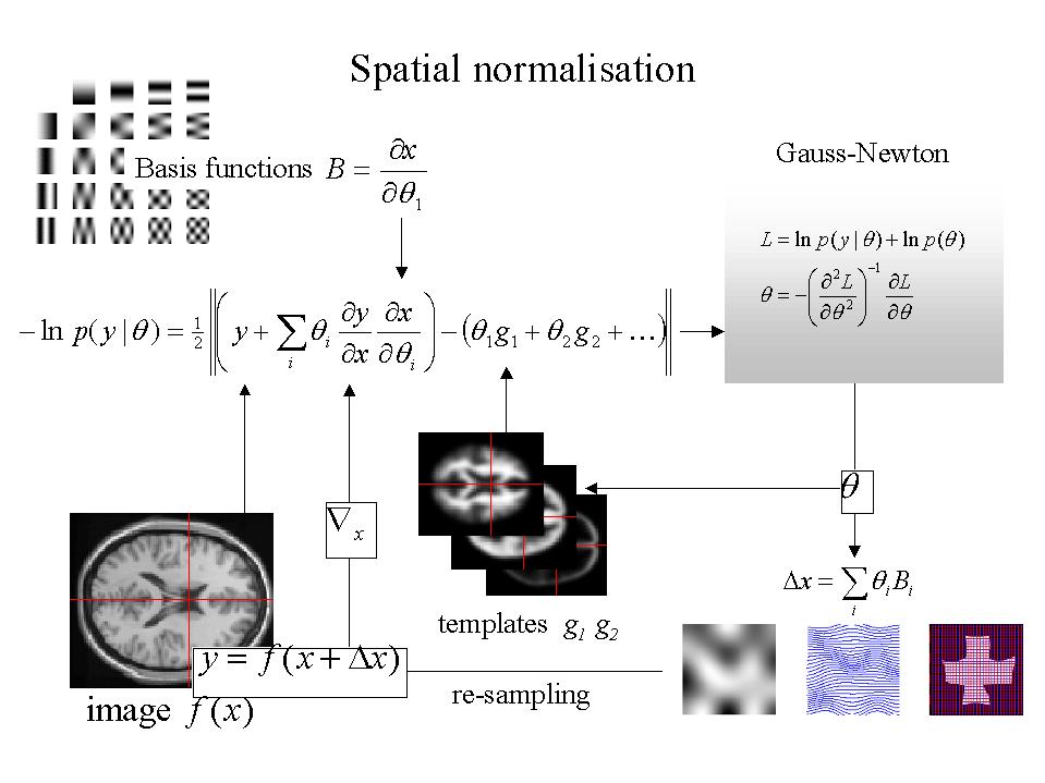
Figure 2. Schematic illustrating a Gauss-Newton scheme for maximizing the posterior probability of the parameters for spatially normalizing an image. This scheme is iterative. At each step the conditional estimate of the parameters is obtained by jointly minimizing the likelihood and the prior potentials. The former is the difference between a resampled (i.e. warped) version y of the image f and the best linear combination of some templates g. These parameters are used to mix the templates and resample the image to progressively reduce both the spatial and intensity differences. After convergence the resampled image can be considered normalized.

3.4 Co-registration of functional and anatomical data

It is sometimes useful to co-register functional and anatomical images. However, with echo-planar imaging, geometric distortions of T₂* images, relative to anatomical T₁-weighted data, are a particularly serious problem because of the very low frequency per point in the phase encoding direction. Typically for echo-planar fMRI magnetic field inhomogeneity, sufficient to cause dephasing of 2? through the slice, corresponds to an in-plane distortion of a voxel. 'Unwarping' schemes have been proposed to correct for the distortion effects (Jezzard and Balaban 1995). However, this distortion is not an issue if one spatially normalizes the functional data.

3.5 Spatial smoothing

The motivations for smoothing the data are fourfold: (i) By the matched filter theorem, the optimum smoothing kernel corresponds to the size of the effect that one anticipates. The spatial scale of hemodynamic responses is, according to high-resolution optical imaging experiments, about 2 to 5mm. Despite the potentially high resolution afforded by fMRI an equivalent smoothing is suggested for most applications. (ii) By the central limit theorem, smoothing the data will render the errors more normal in their distribution and ensure the validity of inferences based on parametric tests. (iii) When making inferences about regional effects using Gaussian random field theory (see Section IV) one of the assumptions is that the error terms are a reasonable lattice representation of an underlying and smooth Gaussian field. This necessitates smoothness to be substantially greater than voxel size. If the voxels are large, then they can be reduced by sub-sampling the data and smoothing (with the original point spread function) with little loss of intrinsic resolution. (iv) In the context of inter-subject averaging it is often necessary to smooth more (e.g. 8 mm in fMRI or 16mm in PET) to project the data onto a spatial scale where homologies in functional anatomy are expressed among subjects.