|
Statistical Parametric Mapping |
|
|
Karl J Friston |
|
|
Wellcome Dept. of Imaging Neuroscience |
In this section we consider some issues that are generic to brain mapping studies that have repeated measures or replications over subjects. The critical issue is whether we want to make an inference about the effect in relation to the within-subject variability or with respect to the between subject variability. For a given group of subjects, there is a fundamental distinction between saying that the response is significant relative to the variability with which that response in measured and saying that it is significant in relation to the inter-subject variability. This distinction relates directly to the difference between fixed and random-effect analyses. The following example tries to make this clear. Consider what would happen if we scanned six subjects during the performance of a task and baseline. We then constructed a statistical model, where task-specific effects were modelled separately for each subject. Unknown to us, only one of the subjects activated a particular brain region. When we examine the contrast of parameter estimates, assessing the mean activation over all the subjects, we see that it is greater than zero by virtue of this subject's activation. Furthermore, because that model fits the data extremely well (modelling no activation in five subjects and a substantial activation in the sixth) the error variance, on a scan to scan basis, is small and the T statistic is very significant. Can we then say that the group shows an activation? On the one hand we can say, quite properly, that the mean group response embodies an activation but clearly this does not constitute an inference that the group's response is significant (i.e. that this sample of subjects shows a consistent activation). The problem here is that we are using the scan to scan error variance and this is not necessarily appropriate for an inference about group responses. In order to make the inference that the group showed a significant activation one would have to assess the variability in activation effects from subject to subject (using the contrast of parameter estimates for each subject). This variability now constitutes the proper error variance. In this example the variance of these six measurements would be large relative to their mean and the corresponding T statistic would not be significant.
The distinction, between the two approaches above, relates to how one computes the appropriate error variance. The first represents a fixed-effect analysis and the second a random-effect analysis (or more exactly a mixed-effects analysis). In the former the error variance is estimated on a scan to scan basis, assuming that each scan represents an independent observation (ignoring serial correlations). Here the degrees of freedom are essentially the number of scans (minus the rank of the design matrix). Conversely, in random-effect analyses, the appropriate error variance is based on the activation from subject to subject where the effect per se constitutes an independent observation and the degrees of freedom fall dramatically to the number of subjects. The term 'random-effect' indicates that we have accommodated the randomness of differential responses by comparing the mean activation to the variability in activations from subject to subject. Both analyses are perfectly valid but only in relation to the inferences that are being made: Inferences based on fixed-effects analyses are about the particular subject[s] studied. Random-effects analyses are usually more conservative but allow the inference to be generalized to the population from which the subjects were selected.
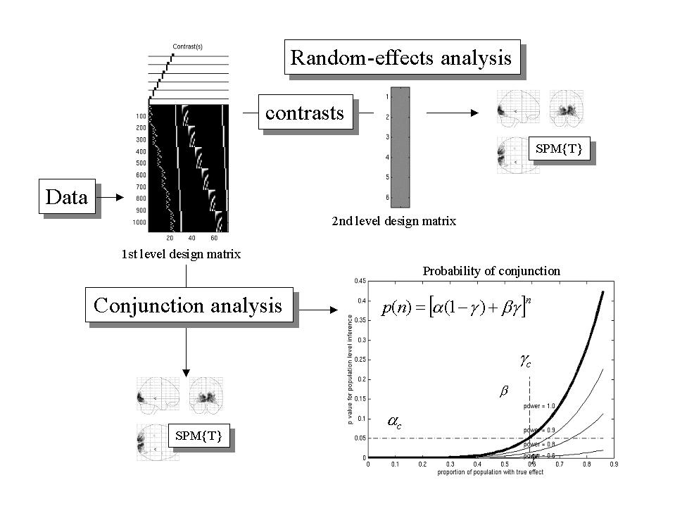
The implementation of random-effect analyses in SPM is fairly straightforward and involves taking the contrasts of parameters estimated from a first-level (fixed-effect) analysis and entering them into a second-level (random-effect) analysis. This ensures that there is only one observation (i.e. contrast) per subject in the second-level analysis and that the error variance is computed using the subject to subject variability of estimates from the first level. The nature of the inference made is determined by the contrasts entered into the second level (see Figure 12). The second-level design matrix simply tests the null hypothesis that the contrasts are zero (and is usually a column of ones, implementing a single sample T test).
The reason this multistage procedure emulates a full mixed-effects analyses, using a hierarchical observation model, rests upon the fact that the design matrices for each subject are the same (or sufficiently similar). In this special case the estimator of the variance at the second level contains the right mixture of variance induced by observation error at the first level and between-subject error at the second. It is important to appreciate this because the efficiency of the design at the first level percolates up to higher levels. It is therefore important to use efficient strategies at all levels in a hierarchical design.
Figure 12. Schematic illustrating the implementation of random-effect and conjunction analyses for population inference. The lower right graph shows the probability p(n) of obtaining a conjunction over n subjects, conditional on a certain proportion ? of the population expressing the effect, for a test with specificity of ? = 0.05, at several sensitivities (? = 1, 0.9, 0.8 and 0.6). The critical specificity for population inference ?c and the associated proportion of the population ?c are denoted by the broken lines.
In some instances a fixed effects analysis is more appropriate, particularly to facilitate the reporting of a series of single-case studies. Among these single cases it is natural to ask what are common features of functional anatomy (e.g. the location of V5) and what aspects are subject-specific (e.g. the location of ocular dominance columns). One way to address commonalties is to use a conjunction analysis over subjects. It is important to understand the nature of the inference provided by conjunction analyses of this sort. Imagine that in 16 subjects the activation in V5, elicited by a motion stimulus, was great than zero. The probability of this occurring by chance, in the same area, is extremely small and is the p-value returned by a conjunction analysis using a threshold of p = 0.5 (T = 0) for each subject. This result constitutes evidence that V5 is involved in motion processing. However, note that this is not an assertion that each subject activated significantly (we only require the T value to be greater than zero for each subject). In other words, a significant conjunction of activations is not synonymous with a conjunction of significant activations.
The motivations for conjunction analyses, in the context of multi-subject studies are twofold. (i) They provide an inference, in a fixed-effect analysis testing the null hypotheses of no activation in any of the subjects, that can be much more sensitive than testing for the average activation. (ii) They can be extended to make inferences about the population as described next
If, for any given contrast, one can establish a conjunction of effects over n subjects using a test with a specificity of a and sensitivity b, the probability of this occurring by chance can be expressed as a function of g, the proportion of the population that would have activated (see the equation in Figure 12 - lower right panel). This probability has an upper bound ac corresponding to a critical proportion gc that is realized when (the generally unknown) sensitivity is one. In other words, under the null hypothesis that the proportion of the population evidencing this effect is less than or equal to gc, the probability of getting a conjunction over n subjects is equal to, or less than, ac. In short a conjunction allows one to say, with a specificity of ac, that more than gc of the population show the effect in question. Formally, we can view this analysis as a conservative 100(1 - ac)% confidence region for the unknown parameter g. These inferences can be construed as statements about how typical the effect is, without saying that it is necessarily present in every subject.
In practice, a conjunction analysis of a multi-subject study comprises the following steps: (i) A design matrix is constructed where the explanatory variables pertaining to each experimental condition are replicated for each subject. This subject-separable design matrix implicitly models subject by condition interactions (i.e. different condition-specific responses among sessions). (ii) Contrasts are then specified that test for the effect of interest in each subjects to give a series of SPM{T} that can be reported as a series of 'single-case' studies in the usual way. (iii) These SPM{T} are combined at a threshold u (corresponding to the specificity a in Figure 12) to give a SPM{Tmin} (i.e. conjunction SPM). The corrected p-values associated with each voxel are computed as described in Figure 6. These p-values provide for inferences about effects that are common to the particular subjects studied. Because we have demonstrated regionally specific conjunctions, one can also proceed to make an inference about the population from which these subjects came using the confidence region approach described above (see Friston et al 1999b for a fuller discussion).