Beamforming OPM Data¶

About¶

In this tutorial we will introduce how to use a beamformer to source localise data. Beamformers are typically thought of as ‘spatial filters’, such the effect of sensor-level external interference on the source reconstruction is often negligible for most neuroimaging studies. They are useful for low-SNR data. Another advantage of beamformers is that all sources in the brain space don’t have to be modelled simultaneously, which is useful for reconstructing a single location in the brain.

Beamformer equation¶

For a given source \(\theta\), the vector \(w\) which represents the weighted sum of channels which best represent that area is defined as:

\[w^T_{\theta} = [l^T_{\theta}C^{-1}l_{\theta}]^{-1}l^{T}_{\theta}C^{-1},\]

where \(C\) is the covariance matrix of the sensor level recordings, and \(l\) is a vector representing the modelled dipole field pattern for a unit-source at \(\theta\). In DAiSS we need to calculate both the dipole patterns and the covariance matrix before assembling the source reconstruction weights.

Where beamformers might be bad for your data

The mathematic description of beamformers imply there are situations where their use can lead to poor source estimates, the main examples are.

Correlated sources: If two spatially separate sources show a high level of correlation (r>0.7), then beamformers will reject these sources entirely.
Large cortical patches: Beamformers assume sources are highly focal in space, so a source which covers a large area of the cortex will fail to reconstruct well.

Generating OPM data¶

For this tutorial we shall create some sources of auditory activity from scratch. We shall do this in two steps, first we’ll create a blank OPM dataset using spm_opm_sim and then simulate some sources.

Creating a dataset¶

For this simulation we shall create an OPM array with the sensitive axes radial to the surface of the scalp and offset 6.5 mm away (which is roughly how far from the scalp an OPM’s gas cell is from the scalp). We’ll also set it up that there will be 40 trials with a prestimulus window of 0.5 seconds. Note: this cannot yet be done from the batch and so we need to do this as a script.

S = [];
S.fs = 200;
S.nSamples = 300;
S.data = zeros(1,300,40);
S.space = 35;
S.offset = 6.5;
S.wholehead = 0;
S.axis = 1;

D = spm_opm_sim(S);
D = D.timeonset(-0.5);
save(D);

Simulating activity from the auditory cortex¶

Now we have an empty MEG dataset, we need to simulate the activity originating from the auditory areas. This is best done in the GUI but can also be generated as a matlabbatch script.

GUIScript

Start the batch editor (Batch button) on main panel. Then from the dropdown menu SPM: select M/EEG -> Source reconstruction -> Simulation of sources. You will see the following menu:

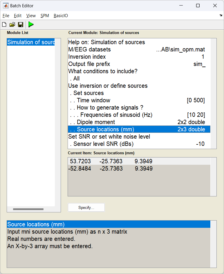
In this example, most of the settings can be left on their defaults for this exercise, but a few have been edited. First the time window has been set to [0 500] ms and the SNR has been lowered to -20 dB.

Don’t forget to update the path with real location of the dataset!

matlabbatch = [];

matlabbatch{1}.spm.meeg.source.simulate.D = {'\path\to\meeg\dataset.mat'};
matlabbatch{1}.spm.meeg.source.simulate.val = 1;
matlabbatch{1}.spm.meeg.source.simulate.prefix = 'sim_';
matlabbatch{1}.spm.meeg.source.simulate.whatconditions.all = 1;
matlabbatch{1}.spm.meeg.source.simulate.isinversion.setsources.woi = [0 500];
matlabbatch{1}.spm.meeg.source.simulate.isinversion.setsources.isSin.foi = [10
                                                                            20];
matlabbatch{1}.spm.meeg.source.simulate.isinversion.setsources.dipmom = [10 10
                                                                        10 5];
matlabbatch{1}.spm.meeg.source.simulate.isinversion.setsources.locs = [53.7203 -25.7363 9.3949
                                                                    -52.8484 -25.7363 9.3949];
matlabbatch{1}.spm.meeg.source.simulate.isSNR.setSNR = -20;

spm_jobman('run',matlabbatch)

Importing data into DAiSS¶

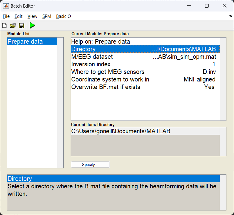
After preprocessing the data, it is ready to enter the DAiSS pipeline. We want the data’s coordinate system to be MNI-aligned (default). This is useful for group analyses as this will mean that exported results will be in or based on MNI coordinates, so no post-registration is required to get all subjects in the same space.

GUIScript

Start the batch editor (Batch button) on main panel. Then from the dropdown menu SPM select Tools -> DAiSS (beamforming) -> Prepare data. You will see the following menu:

Most of the options can be left on their defaults for this example.

Note

The option S.dir in bf_wizard_data requires just the path to where the resultant ‘BF.mat’ file will reside (in this case /path/to/results). For this example we’ve used spm_file to extract this from the variable path_bf.

path_D = '\path\to\meeg\sim_dataset.mat';
path_BF = '\path\to\results\BF.mat';

S = [];
S.D = path_D;
S.dir = spm_file(path_BF,'path');
S.overwrite = 1;

matlabbatch = bf_wizard_data(S);

spm_jobman('run',matlabbatch)

Upon a successful import a file called BF.mat will be created in the target directory.

Specifying a source space¶

The sources module of DAiSS has two roles. First to specify where our sources we want to analyse exist, and second do generate our dipole field patterns associated with sources in a given position and orientation (the \(l\) in our beamformer equation). Here we are going to generate a volumetric grid with sources spaced 5 mm apart from each other. At each location we shall also model three orthogonal dipoles which we we combine later to make one source.

GUIScript

Start the batch editor (Batch button) on main panel. Then from the dropdown menu SPM select Tools -> DAiSS (beamforming) -> Define sources. You will see the following menu:

path_BF = '\path\to\results\BF.mat';

S = [];
S.BF = path_BF;
S.method = 'grid';
S.(S.method).resolution = 5;

matlabbatch = bf_wizard_sources(S);

spm_jobman('run',matlabbatch)

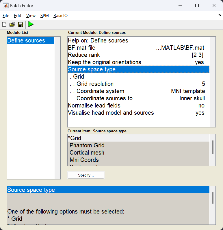
What dipole model are we using?

In this specific example we are using the Single Shell model as described in Guido Nolte’s 2003 Phys. Med. Biol. paper. This partly models the brain as a sphere and then corrects the model based on the shape of the brain/CSF boundary. For MEG data this generates results very similar to complex Boundary Element Models and is currently the recommended dipole model for MEG in SPM.

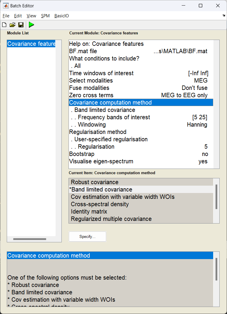
Generating the covariance matrix¶

With the forward model computed, (the \(l\) in our beamformer equation) we can now now focus on the the second variable, the data covariance matrix \(C\). Here we use the features block of DAiSS to filter our data into a target frequency band of choice and then generate a then covariance matrix. In this simulation the matrix we generate will also be regularised to minimise the effect of the covariance matrix can have on the beamforming.

GUIScript

Start the batch editor (Batch button) on main panel. Then from the dropdown menu SPM select Tools -> DAiSS (beamforming) -> Covariance features. You will see the following menu:

S = [];
S.BF = path_BF;
S.method = 'cov';
S.conditions = 'all';
S.(S.method).woi = [Inf Inf]; % Uses the whole trial
S.(S.method).foi = [5 25]; 
S.reg = 'manual'; 
S.(S.reg).lambda = 5; % 5 percent regularisation.

matlabbatch = bf_wizard_features(S);

spm_jobman('run',matlabbatch)

Why regularisation can be important

If we look at the beamformer equation at the start of this tutorial, you might notice that we don’t use the covariance matrix as calculated, but rather the inverse \(C^{-1}\). Inverting a matrix requires that two properties of the matrix, the condition and rank are optimal. The condition is the ratio of the largest-to-smallest singular values in the matrix and will dictate the range of values, if this is too large, this will lead to the smallest values (which often correspond to the noise) dominating when we invert the matrix. Similarly the rank of the data quantifies the number of independent measures in the matrix, and if this is lower than the number of channels used to make the matrix then this will make the condition of the matrix explode. Regularisation attempts to ultimately reduce the condition of the matrix to avoid this problem.

What kind of regularisation are we doing here?

Tikhonov regularisation. This is a relatively simple regularisation method we we load the diagonal elements of the covariance matrix to reduce the overall condition. Here \(C_{\text{reg}}=C+\mu I\), where \(I\) is an identity matrix and \(\mu\) is the regularisation parameter. In this case we’ve asked for lambda to be 5, but what is lambda and this 5 is of what exactly? In DAiSS this represents the percentage of average power over all the sensors in the time-frequency window we estimate the covariance, this is calculated using the average of the trace of the covariance \(\mu=0.01\times\lambda\times\text{tr}(C)/N\) where \(N\) is the number of channels.

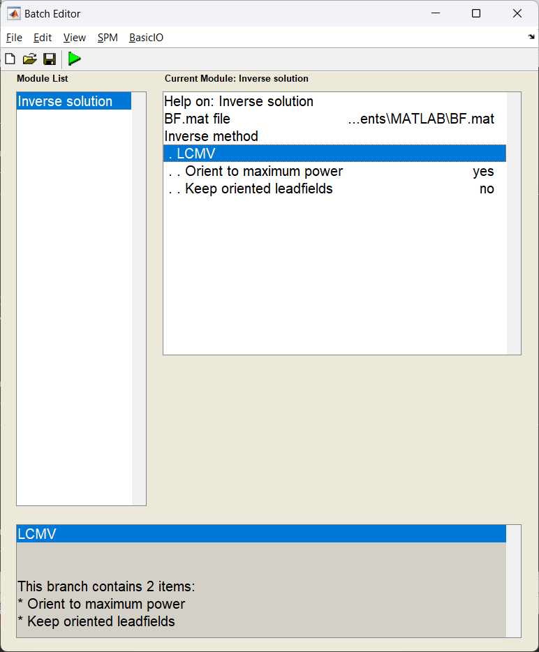
Source inversion¶

This is the point where the beamforming calculation happens. Having calculated our covariance and dipole models, we can combine them using the beamformer equation.

GUIScript

Start the batch editor (Batch button) on main panel. Then from the dropdown menu SPM select Tools -> DAiSS (beamforming) -> Inverse solution. You will see the following menu:

S = [];
S.BF = path_BF;
S.method = 'lcmv';

matlabbatch = bf_wizard_inverse(S);

spm_jobman('run',matlabbatch)

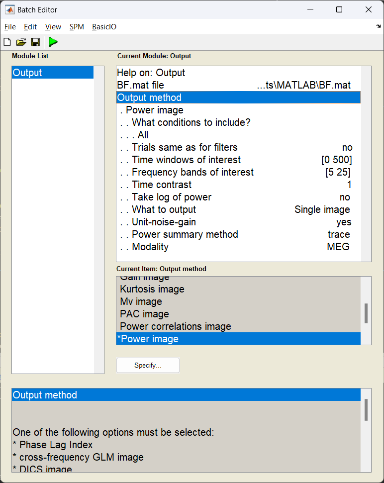
Source power estimation¶

With the source weight vectors calculated, we can now estimate the power for a given source in and time-frequency window of our choosing. In this case this will be during the “stimulus” period and within the frequency bands we calculated our covariance matrix with. We shall also perform a depth correction, as beamformers tend to bias their variance towards the centre of the brain without it.

GUIScript

Start the batch editor (Batch button) on main panel. Then from the dropdown menu SPM select Tools -> DAiSS (beamforming) -> Output. You will see the following menu:

S = [];
S.BF = path_BF;
S.conditions = 'all';
S.woi = [0 500]; % pre-stim and during
S.foi = [5 25];
S.contrast = 1;
S.method = 'image_power';
S.(S.method).scale = 1; 
matlabbatch = bf_wizard_output(S);

spm_jobman('run',matlabbatch)

How beamformer power is calculated

For a given source \(\theta\), the power \(P_{\theta}\) is calculated using \(P_{\theta} = w_{\theta}^TCw_{\theta}\)

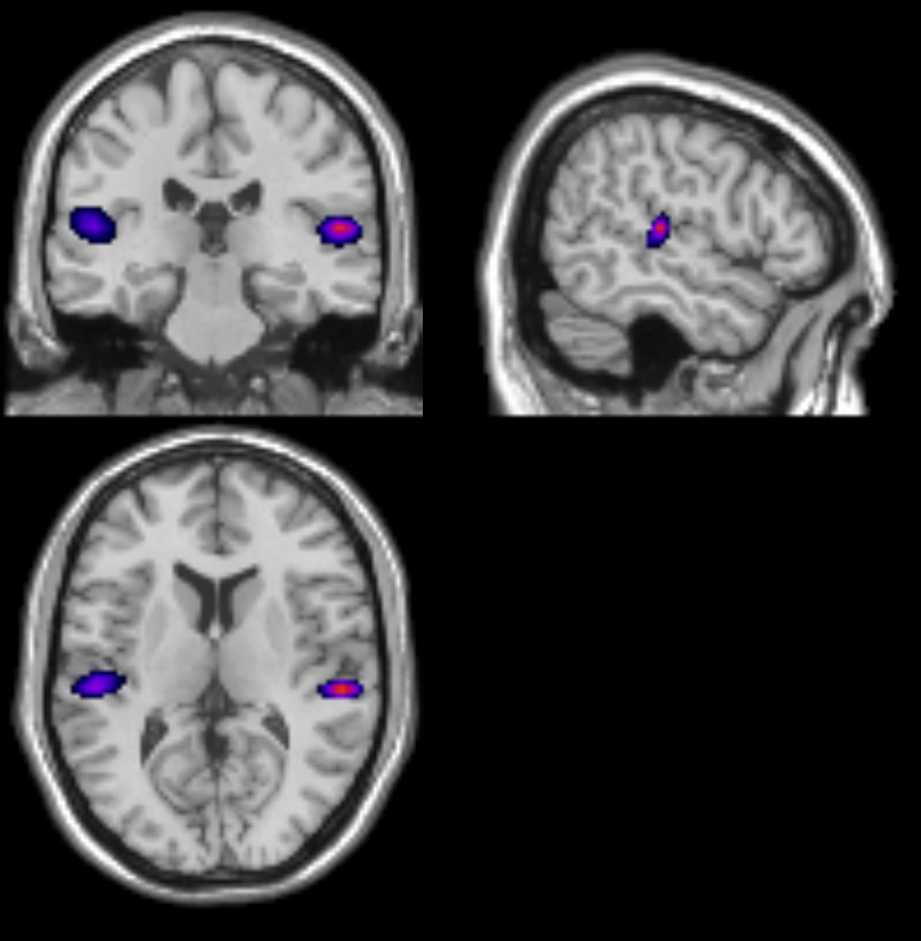
Viewing the results¶

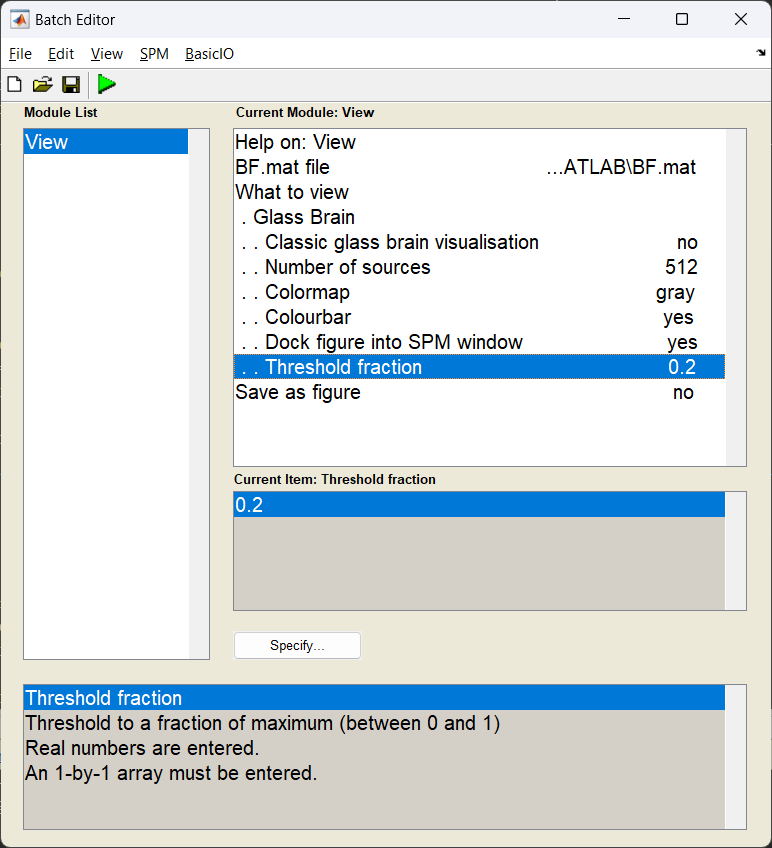
Before writing out the results to disk, it is possible to plot some outputs. image_power is one such example. To view a glass brain plot showing where the largest amount of power was reconstructed:

GUICode

Start the batch editor (Batch button) on main panel. Then from the dropdown menu SPM select Tools -> DAiSS (beamforming) -> View. You will see the following menu:

S = [];
S.BF = path_BF;
S.method = 'glass';
S.(S.method).classic = 0; % set to 0 for new plotter
S.(S.method).threshold = 0.2;

matlabbatch = bf_wizard_view(S);

spm_jobman('run',matlabbatch)

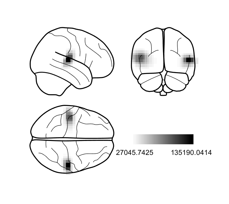
If all has gone well, then we should see two sources originating from approximately the primary auditory cortices!

Help! All my power is in the centre of the brain!

Does your power image look like below?

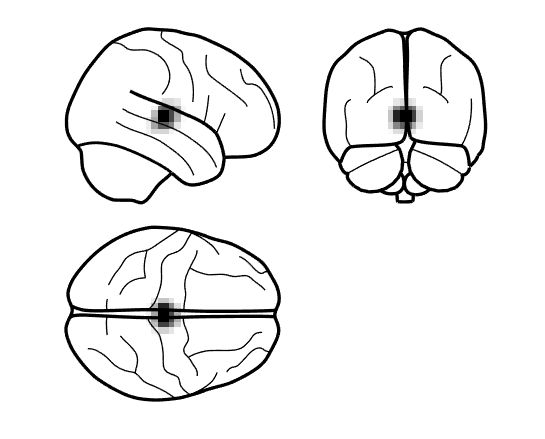
This can happen if you do not depth normalise your beamformed data. When generating the power image, ensure the depth correction is turned on using S.image_power.scale = 1; when using code or set the option of unit-noise-gain to yes in the batch.

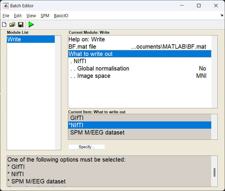
Exporting results¶

We can now export the power image as a NIfTI file so it can be shared with other software, or entered into a second-level group analysis in SPM with other subjects.

GUICode

Start the batch editor (Batch button) on main panel. Then from the dropdown menu SPM select Tools -> DAiSS (beamforming) -> Write. You will see the following menu:

S = [];
S.BF = path_BF;
S.method = 'nifti';

matlabbatch = bf_wizard_write(S);

spm_jobman('run',matlabbatch)

Overlaid power image on a template anatomical in MRIcron