Multimodal, Multisubject data fusion
Evoked analysis
At this point, the preprocessing forks into two strands: one for trial-averaged amplitude analysis and one for time-frequency analysis. The first of these corresponds to a typical evoked response (ER) analysis, where we simply average across trials in each condition (note this will attenuate any non-phase locked, i.e. induced responses; to detect these, we will later perform time-frequency analysis before averaging). Before averaging though, we will crop the 400ms buffer around each trial (which is only necessary for the time-frequency analysis).
Crop
To crop the data, select the crop option from “SPM – M/EEG –
Preprocessing – Crop”. Select the datafile called
Mcbdespmeeg_run_01_sss.mat produced from the final EEG re-referencing
(“Montage”) step above. A 100ms pre-stimulus baseline period is normally
sufficient, and we do not care about responses after 800ms for this
particular analysis, so we can cut off 400ms at the start and end of
each trial to produce an epoch from -100ms to +800ms. To do this, select
“Time Window” from the “Current Module” window, then the “Specify”
button. Within the pop up window, enter [-100 800] as a 1-by-2 array.
The channel selection will be “all”. This file output will be prepended
with a p.
Artefact detection
There are many ways to define artifacts (including special toolboxes;
see other SPM manual chapters). Here we focus on just one simple means
of detecting blinks by thresholding the EOG channels. Select “Artefact
detection” from the “SPM – M/EEG – Preprocessing” menu. For the input
file, select a dependency on the output of the previous step (“Crop”).
Next, select “New: Method” from the box titled “Current Item: How to
look for artefacts”. Back in the “Current Module” window, highlight
“Channel selection” to list more options, choose “Select channels by
type” and select “EOG”. Then do not forget to also delete the default
“All” option! Then press the “\(<\)-X” to select “threshold channels”,
click the “Specify” button and set this to 200 (in units of
microvolts). The result of this thresholding will be to mark a number of
trials as “bad” (these can be reviewed after the pipeline is run if you
like). Bad trials are not deleted from the data, but marked so they will
be excluded from averaging below. The output file will be prepended with
the letter “a”.
Combine Planar Gradiometers
The next step is only necessary for scalp-time statistics on planar
gradiometers. For scalp-time images, one value is needed for each sensor
location. Neuromag’s planar gradiometers measure two orthogonal
directions of the magnetic gradient at each location, so these need to
be combined into one value for a scalar (rather than vector) topographic
representation. The simplest way to do this is to take the Root Mean
Square (RMS) of the two gradiometers at each location (i.e. estimate the
2D vector length). In SPM, this will create a new sensor type called
MCOMB. Note that this step is NOT necessary for source reconstruction
(where, the forward model captures both gradiometers). Note also that
the RMS is a nonlinear operation, which means that zero-mean additive
noise will no longer cancel by averaging across trials, in turn meaning
that it is difficult to compare conditions that differ in the number of
trials. To take the RMS, select “Combine Planar” from the “SPM – M/EEG
– Preprocessing” menu, highlight “File Name”, select the “dependency”
button, and choose the Artefact-corrected file above. Leave the “copying
mode” as default – “Replace planar”. The produced file will be
prepended with P.
Trial averaging
To average the data across trials, select “SPM – M/EEG – Average –
Averaging”, and define the input as dependent on the output of the
planar combination module. Keep the remaining options as the default
values. (If you like, you could change the type of averaging from
“standard” to “Robust”. Robust averaging is a more sophisticated version
of normal averaging, where each timepoint in each trial is weighted
according to how different it is from the median across trials. This can
be a nice feature of SPM, which makes averaging more robust to atypical
trials, though in fact it does not make much difference for the present
data, particularly given the large numbers of trials, and we do not
choose it here simply because it takes much longer than conventional
averaging.) Once completed, this file will have a prefix of m.
Contrasting conditions
We can also take contrasts of our trial-averaged data, e.g., to create a
differential ER between faces and scrambled faces. This is sometimes
helpful to see condition effects, and plot their topography. These
contrasts are just linear combinations of the original conditions, and
so correspond to vectors with 3 elements (for the 3 conditions here).
Select “SPM – M/EEG – Average – Contrast over epochs”, and select the
output of “Averaging” above as in the dependent input. You can then
select “New Contrast” and enter as many contrasts as you like. The
resulting output file is prepended with w.
For example, to create an ER that is the difference between faces
(averaged across Famous and Unfamiliar) and scrambled faces, enter the
vector [0.5 0.5 -1] (assuming conditions are ordered
Famous-Unfamiliar-Scrambled; see comment earlier in “Prepare” module),
and give it a name. Or to create the differential ER between Famous and
Unfamiliar faces, enter the vector [1 -1 0]. Sometimes it is worth
repeating the conditions from the previous averaging step by entering,
in this case, three contrasts: [1 0 0], [0 1 0] and [0 0 1], for
Famous, Unfamiliar and Scrambled conditions respectively. These will be
exactly the same as in the averaged file above, but now we can examine
them, as well as the differential responses, within the same file (i.e.
same graphics window when we review that file), and so can also delete
the previous m file.
Save batch and review.
At this point, you can save batch and script again. The resulting batch
file should look like the batch_preproc_meeg_erp_job.m file in the
SPM12batch part of the SPMscripts FTP directory. The script file can
be run (and possibly combined with the previous script created).
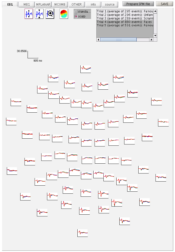
We will start by looking at the trial-averaged ERs to each of the three
conditions. Select the “Display” button on the SPM Menu and select the
file wmPapMcbdspmeeg_run_01_sss.mat. Then select, for example, the
“EEG” tab, and you will see each channel as a row (“strip”, or “standard
view”) for the mean ER for Famous faces. If you press “scalp” instead,
the channels will be flat-projected based on their scalp position (nose
upwards). You can now display multiple conditions at once by holding the
shift-key and selecting Trials 2 and 3 (Unfamiliar and Scrambled) as
well (as in Figure 1.2, after zooming the y-axis
slightly). If you press the expand y-axis button (top left) a few times
to up-scale the data, you should see something like in
Figure 1.2. You can see the biggest evoked
potentials (relative to average over channels) at the back of the head.
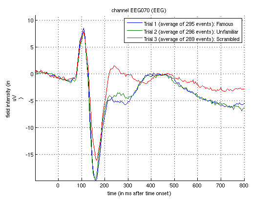
If you press the magnifying glass icon, then with the cross-hairs select Channel 70 (in bottom right quadrant of display), you will get a new figure like in Figure 1.3 that shows the ERPs for that channel in more detail (and which can be adjusted using the usual MATLAB figure controls). You can see that faces (blue and green lines) show a more negative deflection around 170ms than do scrambled faces (red line), the so-called “N170” component believed to index the earliest stage of face processing.
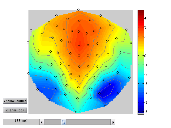
To see the topography of this differential N170 component, select instead the fourth trial (contrast) labelled “Faces – Scrambled”. Then press the coloured topography icon, and you will get a new figure with the distribution over the scalp of the face-scrambled difference. If you shift the time-slider on the bottom of that window to the leftmost position, and then repeatedly click on the right arrow, you will see the evolution of the face effect, with no consistent difference during the prestimulus period, or until about 155ms, at which point a clear dipolar field pattern should emerge (Figure 1.4).
You can of course explore the other sensor-types (magnetometers, MEG) and combined gradiometers (MCOMB), which will show an analogous “M170”. You can also examine the EOG and ECG channels, which appear under the “OTHER” tab. (Note that the VEOG channel contains a hint of an evoked response: this is not due to eye-movements, but due to the fact that bipolar channels still pick up a bit of brain activity too. The important thing is that there is no obvious EOG artefact associated with the difference between conditions, such as differential blinks.)
But how do we know whether this small difference in amplitude around 150-200ms is reliable, given the noise from trial to trial? And by looking at all the channels and timepoints, in order to identify this difference, we have implicitly performed multiple comparisons across space and time: so how do we correct for these multiple comparisons (assuming we had no idea in advance where or when this face-related response would occur)? We can answer these questions by using random field theory across with scalp-time statistical parametric maps. But first, we have to convert these sensor-by-time data into 3D images of 2D-location-by-time.
Time-Sensor images
To create 3D scalp-time images for each trial, the 2D representation of
the scalp is created by projecting the sensor locations onto a plane,
and then interpolating linearly between them onto a 32\(\times\)32
pixel grid. This grid is then tiled across each timepoint. To do this,
you need to select the “SPM – M/EEG – Images – Convert2Images” option
in the batch editor. For the input file, select the
PapMcbdspmeeg_run_01_sss.mat file that contains every cropped trial
(i.e, before averaging), but with bad trials marked (owing to excessive
EOG signals; see earlier). Next select “Mode”, and select “scalp x
time”. Then, select “conditions”, select “Specify” and enter the
condition label “Famous”. Then repeat for the condition labels
“Unfamiliar” and “Scrambled”.
To select the channels that will create your image, highlight the
“Channel selection”, and then select “New: Select channels by type” and
select “EEG”. The final step is to name the Directory prefix
eeg_img_st this can be done by highlighting “directory prefix”,
selecting “Specify”, and the prefix can then be entered.
This process can be repeated for the MEGMAG channels, and the MEGCOMB
channels (although we will focus only on the EEG here). If so, the
easiest way to do this is to right-click “Convert2Images” in the Module
List, and select “replicate module”. You will have to do this twice, and
then update the channels selected, and the directory prefix to
mag_img_mat and grm_img_mat to indicate the magnetometers (MEGMAG)
and the gradiometers (MEGCOMB) respectively.
Save batch and review.
At this point, you can save batch and script again. The resulting batch
file should look like the batch_preproc_meeg_erp_images_job.m file in
the SPM12batch FTP directory. Once you have run this script, a new
directory will be created for each channel-type, which is based on the
input file and prefix specified above (e.g.,
eeg_img_st_PapMcbdspmeeg_run_01_sss for the EEG data). Within that
directory will be three 4D NIfTI files, one per condition. It is very
important to note that these 4D files contain multiple “frames” (i.e. 3D
scalp-time images), one per trial (i.e. 296 in the case of unfamiliar
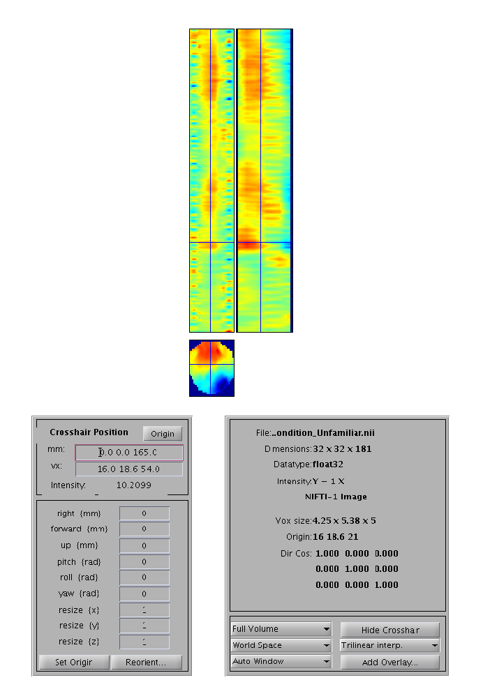
faces). To view one of these, press “Display – Images” in the SPM Menu
window, and select, say, the condition_Unfamiliar.nii file. But note
that by default you will only see the first scalp-time image in each
file (because the default setting of “Frames” within the Select Image
window is 1). To be able to select from all frames, change the
“Frames” value from 1 to Inf (infinite), and now you will see all
296 frames (trials) that contained Unfamiliar faces. If you select, say,
number 296, you should see an image like in
Figure 1.5 (this was created after selecting
“Edit – Colormap” from the top toolbar, then “Tools – Standard
Colormap – Jet”, and entering [0 0 165] as the coordinates in order
to select 165ms post-stimulus). You can scroll will the cross-hair to
see the changes in topography over time.
Note that Random Field Theory, used to correct the statistics below, assumes a certain minimum smoothness of the data (at least three times the voxel size). The present data meet this requirement, but in other cases, one could add an additional step of Gaussian smoothing of the images to ensure this smoothness criterion is met.
Scalp-Time Statistics across trials within one subject
Now we have one image per trial (per condition), we can enter these into a GLM using SPM’s statistical machinery (as if they were fMRI or PET images). If we ignore temporal autocorrelation across trials, we can assume that each trial is an independent observation, so our GLM corresponds to a one-way, non-repeated-measures ANOVA with 3 levels (conditions).
Model Specification
To create this model, open a new batch, select “Factorial design
specification” under “Stats” on the SPM toolbar at the top of the batch
editor window. The first thing is to specify the output directory where
the SPM stats files will be saved. So first create such a directory
within the subject’s sub-directory, calling it for example STStats,
and then create a sub-directory eeg within STStats (and potentially
two more called mag and grm if you want to examine other
sensor-types too). Then go back to the batch editor and select this new
eeg directory.
Highlight “Design” and from the current item window, select “One-way
ANOVA”. Highlight “Cell”, select “New: Cell” and repeat until there are
three cells. Select the option “Scan” beneath each “Cell” heading
(identified by the presence of a “\(<\)-X”). Select “Specify”, and in the
file selector window, remember to change the “Frames” value from 1 to
Inf as previously to see all the trials. Select all of the image files
for one condition (by using the right-click “select all” option). It is
vital that the files are selected in the order in which the conditions
will later appear within the Contrast Manager module (i.e., Famous,
Unfamiliar, Scrambled). Next highlight “Independence” and select “Yes”,
but set the variance to “Unequal”. Keep all the remaining defaults (see
other SPM chapters for more information about these options).
Finally, to make the GLM a bit more interesting, we will add 3 extra
regressors that model the effect of time within each condition (e.g. to
model practice or fatigue effects). (This step is optional if you’d
rather omit.) Press “New: Covariate” under the “Covariates” menu, and
for the “Name”, enter “Order Famous”. Keep the default “None” to
interactions, and “Overall mean” for “centering”. We now just need to
enter a vector of values for every trial in the experiment. These trials
are ordered Famous, Unfamiliar and Scrambled, since this is how we
selected them above. So to model linear effects of time within Famous
trials, we need a vector that goes from 1:295 (since there are 295
Famous trials). However, we also need to mean-correct this, so we can
enter detrend([1:295],0) as the first part of the vector (covariate)
required. We then need to add zeros for the remaining Unfamiliar and
Scrambled trials, of which there are 296+289=585 in total. So the
complete vector we need to enter (for the Famous condition) is
[detrend([1:295],0) zeros(1,585)]. We then need to repeat this time
covariate for the remaining two conditions. So press “New: Covariate”
again, but this time enter “Order Unfamiliar” as the name, and
[zeros(1,295) detrend([1:296],0) zeros(1,289)] as the vector. Finally,
press “New: Covariate”, but this time enter “Order Scrambled” as the
name, and [zeros(1,591) detrend([1:289],0)] as the vector.
This now completes the GLM specification, but before running it, we will add two more modules.
Model Estimation
The next step within this pipeline is to estimate the above model. Add a module for “Model Estimation” from the “Stats” option on the SPM toolbar and define the file name as being dependent on the results of the factorial design specification output. For “write residuals”, keep “no”. Select classical statistics.
Setting up contrasts
The final step in the statistics pipeline is create some planned
comparisons of conditions by adding a “Contrast Manager” module from the
“Stats” bar. Define the file name as dependent on the model estimation.
The first contrast will be a generic one that tests whether significant
variance is captured by the 6 regressors (3 for the main effect of each
condition, and 3 for the effects of time within each condition). This
corresponds to an F-contrast based on a 6x6 identity matrix. Highlight
contrast sessions and select a new F-contrast session. Name this
contrast “All Effects”. Then define the weights matrix by typing in
eye(6) (which is MATLAB for a 6\(\times\)6 identity matrix).
(Since there is only one “session” in this GLM, select “Don’t replicate”
from the “replicate over sessions” question.) We will use this contrast
later to plot the parameter estimates for these 6 regressors.
More interestingly perhaps, we can also define a contrast that compares
faces against scrambled faces (e.g. to test whether the N170 seen in the
average over trials in right posterior EEG channels in
Figure 1.3 is reliable given the variability
from trial to trial, and to also discover where else in space or time
there might be reliable differences between faces and scrambled faces).
So make another F-contrast, name this one “Faces (Fam+ Unf) \(<>\)
Scrambled”, and type in the weights [0.5 0.5 -1 0 0 0] (which
contrasts the main effect of faces vs scrambled faces, ignoring any time
effects (though SPM will complete the final zeros if you omit). Note
that we use an F-test because we don’t have strong interest in the
polarity of the face-scrambled difference (whose distribution over the
scalp depends on the EEG referencing). But if we did want to look at
just positive and negative differences, you could enter two T-contrasts
instead, with opposite signs on their weights.
Save batch and review
Once you have added all the contrasts you want, you can save this batch
file (it should look like the batch_stats_ANOVA_job.m file in the
SPM12batch FTP directory). This only runs a GLM for one sensor-type
(we cannot combine the sensors until we get to source space later), so
you can write a script around this batch that calls it three times, once
per sensor-type (i.e, for magnetometers and gradiometer RMS too), just
changing the output directory and input files (see master_script.m on
the SPM12batch FTP directory).
The results of this output can be viewed by selecting “Results” from the
SPM Menu window. Select the SPM.mat file in the STStats/eeg
directory, and from the new “Contrast Manager” window, select the
pre-specified contrast “Faces (Fam+Unf) \(<>\) Scrambled”. Within the
Interactive window which will appear on the left hand side, select the
following: Apply Masking: None, P value adjustment to control: FWE, keep
the threshold at 0.05, extent threshold {voxels}: 0; Data Type:
Scalp-Time. The Graphics window should then show what is in
Figure 1.6.
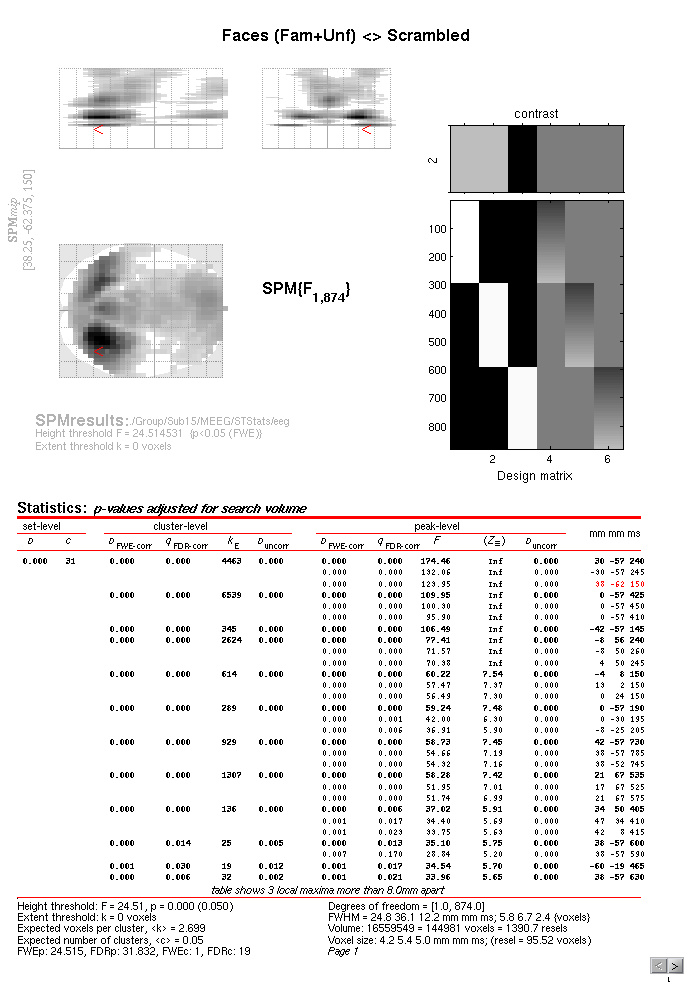
If you move the cursor to the earliest local maximum – the third local
peak in the first cluster – this corresponds to x=+38mm, y=-62mm
and t=150ms (i.e. right posterior scalp, close to the sensor shown in
Figure 1.3, though note that distances are
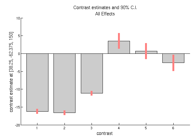
only approximations). If you then press “Plot – Contrast Estimates –
All Effects”, you will get 6 bars like in
Figure 1.7. The first three reflect the three
main conditions (the red bar is the standard error from the model fit).
You can see that Famous and Unfamiliar faces produce a more negative
amplitude at this space-time point than Scrambled faces (the “N70”). The
next three bars show the parameter estimates for the modulation of the
evoked response by time. These effects are much smaller relative to
their error bars (i.e., less significant), but suggest that the N170 to
Famous faces becomes less negative with time, and that to scrambled
faces becomes larger (though one can test these claims formally with
further contrasts).
There are many further options you can try. For example, within the
bottom left window, there will be a section named “Display”, in the
second drop-down box, select “Overlay – Sections” and from the browser,
select the mask.nii file in the analysis directory. You will then get
a clearer image of suprathreshold voxels within the scalp-time-volume.
Or you can of course examine other contrasts, such as the difference
between famous and unfamiliar faces, which you will see is a much weaker
and slightly later effect.