Modelling parametric responses
Parametric modulators
Before setting up the design matrix, we must first load into MATLAB the
Stimulus Onsets Times (SOTs), as before, and also the “Lags”, which are
specific to this experiment, and which will be used as parametric
modulators. The Lags code, for each second presentation of a face (N2
and F2), the number of other faces intervening between this (repeated)
presentation and its previous (first) presentation. Both SOTs and Lags
are represented by MATLAB cell arrays, stored in the sots.mat file.
- At the MATLAB command prompt type
load sots. This loads the stimulus onset times and the lags (the latter in a cell array calleditemlag.
Model specification
Now press the Specify 1st-level button.
This will call up the specification of a fMRI specification job in the
batch editor window. Then:
-
Press
FileandLoad batch, select thecategorical_spec.matjob file you created earlier. -
Open
Conditionsand then open the secondCondition. -
Highlight
Parametric Modulations, selectNew Parameter. -
Highlight
Nameand enterLag, highlight values and enteritemlag{2}, highlight polynomial expansion and2nd order. -
Now open the fourth
ConditionunderConditions. -
Highlight
Parametric Modulations, selectNew Parameter. -
Highlight
Nameand enterLag, highlightvaluesand enteritemlag{4}, highlightpolynomial expansionand2nd order. -
Open
Canonical HRFunderBasis Functions, highlightModel derivativesand selectNo derivatives(to make the design matrix a bit simpler for present purposes!). -
Highlight
Directoryand selectDIR/parametric(having “unselected” the currently defined folder from the Categorical analysis). -
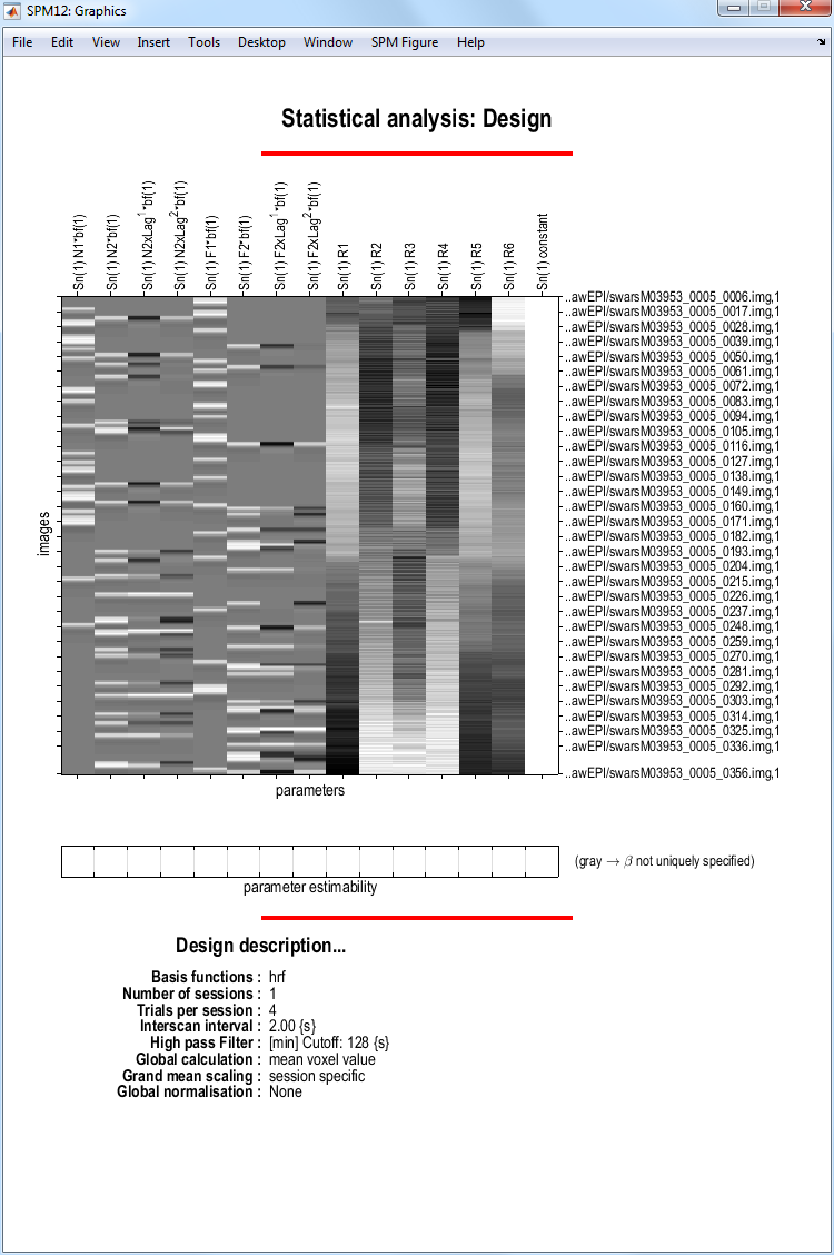
Save the job as
parametric_specand press theRunbutton.
This should produce the design matrix shown below.
Model estimation
Press the Estimate button. This will call
up the specification of an fMRI estimation job in the batch editor
window. Then
-
Highlight the
Select SPM.matoption and then choose theSPM.matfile saved in theDIR/parametricfollder. -
Save the job as
parametric_est.joband press theRunbutton.
SPM will write a number of files into the selected folder (directory) including
an SPM.mat file.
Plotting parametric responses
We will look at the effect of lag (up to second order, ie using linear and quadratic terms) on the response to repeated Famous faces, within those regions generally activated by faces versus baseline. To do this
-
Press
Resultsand select theSPM.matfile in theDIR/parametricfolder. -
Press
Define new contrast, enter the nameFamous Lag, press theF-contrastradio button, enter1:6 9:15in thecolumns in reduced designwindow, presssubmit,OKandDone. -
Select the
Famous Lagcontrast. -
Apply masking ? [None/Contrast/Image]
- Specify
Contrast.
- Specify
-
Select the
Positive Effect of Condition 1T contrast.- Change to an
0.05uncorrected mask p-value.
- Change to an
-
Nature of Mask ?
inclusive. -
p value adjustment to control: [FWE/none]
- Select
None.
- Select
-
Threshold {F or p value}
- Accept the default value,
0.001.
- Accept the default value,
-
Extent threshold {voxels} [0]
- Accept the default value,
0.
- Accept the default value,
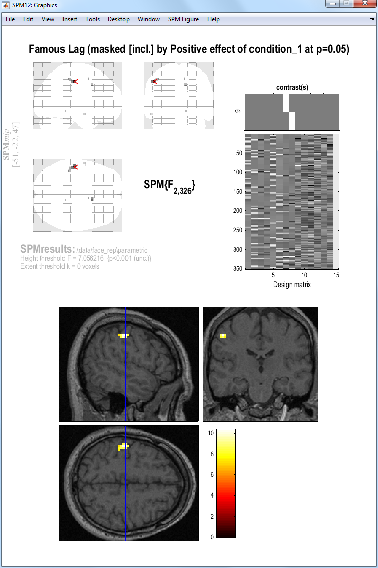
The figure below shows the MIP and an overlay of
this parametric effect using overlays, sections and selecting the
wmsM03953_0007.nii image.
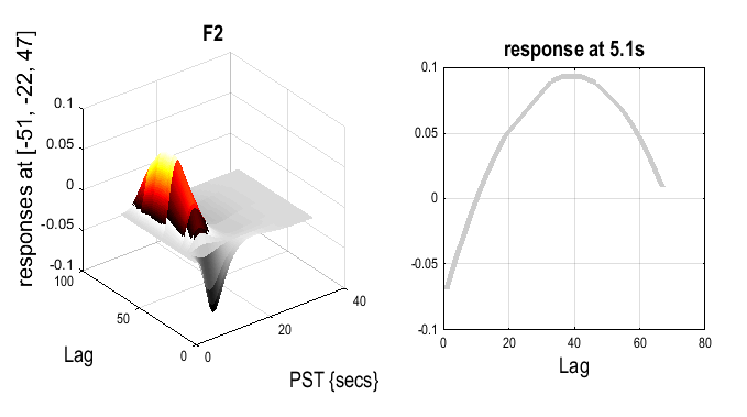
To plot the effect in the time domain:
-
Right clicking on the MIP and selecting
global maxima. -
Pressing
Plot, and selectingparametric responsesfrom the pull-down menu. -
Which effect ? select
F2.
This shows a quadratic effect of lag, in which the response appears negative for short-lags, but positive and maximal for lags of about 40 intervening faces (note that this is a very approximate fit, since there are not many trials, and is also confounded by time during the session, since longer lags necessarily occur later (for further discussion of this issue, see the SPM2 example analysis of these data on the webpage).