Sensor level: Evoked response pipeline
Introduction
This page goes through an example preprocessing pipeline for a sensor-level evoked response analysis. The data used can be downloaded here.
Data import
Currently SPM supports a file format that has the raw data stored in a binary file and all the metadata stored in TSV and JSON files. This is designed to be as aligned as possible to the BIDS file structure. Data from Cerca Magnetics is stored in a similar format and we will analyse such a dataset in this tutorial. The necessary input arguments are the path to the binary file(S.data) and the path to the TSV file that contains the position information(S.positions)
Note
If you would like your file format to be supported by SPM please open an issue on GitHub. Currently supported data formats are documented here.
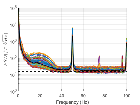
Power Spectral Density
Once OPM data is imported the first step should be to look at the PSD (power spectral density). This plot tells us if any channels are deviating notably from their manufacturer specifications or are clear outlier channels.
Filtering
We can also filter our data to remove very low frequency interference and very high frequency interference.
The key arguments are S.freq which sets the cut-off frequency and S.band which sets the type of filter (high-pass or low-pass)
S=[];
S.D=D;
S.freq=[10];
S.band = 'high';
fD = spm_eeg_ffilter(S);
S = [];
S.D = fD;
S.freq = [70];
S.band = 'low';
fD = spm_eeg_ffilter(S);
S.band argument but we won’t run that here.
Harmonic Models of OPM data
While OPM sensors are sensitive to brain signal they are also incredibly sensitive to environmental interference. Unlike modern MEG systems OPMs come with no built-in interference rejection. As such, all interference must be removed post-hoc using software. Here we will review some principled approaches to removing environmental interference based on solutions to Laplace’s equation.
Spatial models of interference
By solving Laplace’s equation in spherical coordinates we can model OPM interference as a linear combination of vector spherical harmonics. The key arguments are the M/EEG object argument S.D and the order argument S.L. The order argument reflects how complicated the model of interference is. The number of regressors used in the interference model scales as S.L^2+2*S.L. As such, for this method it is recommended to have many more channels than this number. It is generally not recommended to increase the order above S.L=1 for radial samplings of the magnetic field. It is strongly recommended that higher orders are only used for multi-axis OPM systems.
Spatial models of interference and brain signal
If you have an OPM array with more than 120 channels it is possible to not only fit a model of the interference but also a compact model of the brain signal using spheroidal harmonics. The advantage of fitting this additional brain signal model is that as you spatially oversample the data the white noise component of your data will reduce increasing the SNR of the data. Fitting the brain signal model also helps minimise the impact of interference that may be common to just a few channels.
Spatio-temporal models of interference and brain signal
If the source of magnetic interference is quite near the array then the low order spatial models will not be able to remove the interference. This problem is further exacerbated by the presence of sensor non-linearities such as calibration and orientation errors. This kind of interference can be identified using a temporal subspace intersection (implemented using CCA). This step requires setting the argument S.corrLim which is the the threshold (value between 0 and 1) at which one considers two subspaces to have intersected.
How does subspace intersection work?
spm_opm_amm defines 3 subspaces. A brain space using internal spheroidal harmonics (of default order S.li=9), an interference space using external spheroidal harmonics (of default order S.li=2) and an intermediate space that contains the data that is not well modelled by the internal or external harmonics. If the origin of magnetic interference is spatially close by it will not be well modelled by the external harmonics and will be present in the intermediate space. However, due to partial spatial correlation between complex interference and brain signal part of this interference will also be present in the brain signal space. If we assume that over long time scales (5-10s) brain signals (as observed by OPMs) are poorly temporally correlated any high temporal correlations (temporal subspace intersection) between the brain space and the intermediate space are most likely a reflection of magnetic interference. This interference is then readily removed using linear regression.
How do I pick a value for S.corrLim?
Setting a lower value for S.corrLim will result in more aggressive cleaning of the data but will increase the risk of removing interesting brain signal. The factors that influence this decision are the order of the internal harmonics (S.li), the SNR of the brain response, the time scale at which physiological correlations exist, the length of the time window analysed and the number of channels in your array. As such it is not possible to extrapolate any heuristics one might have developed from using other temporal subspace intersection methods such as tSSS. However, the code has been developed so that values greater than 0.98 are generally safe for arrays of less than 200 channels.
How do I choose which model to use?
- If you have less than 120 channels use
spm_opm_hfc. - If you have radial only samplings do not increase
S.Lbeyond 1. - If you have more than 120 channels use
spm_opm_amm. - If you have more than 120 channels and have spatially complex interference use
spm_opm_ammwithS.corrLimset between0.95and1.
Is my data now rank deficient? When does rank matter?
Yes, all these methods reduce the rank of the data. The function spm_opm_hfc reduces the rank by L^2+2L (e.g. order 1 reduces rank by 3, order 2 by 8, order 3 by 15). The function spm_opm_amm reduces the rank to the internal order squared plus twice the internal order (S.li^2+2*S.li). By default the internal order is set to 9 which amounts to setting the rank of the data to 99. Reducing the rank of the data involves setting the contribution of certain spatial components (hopefully interference) to zero. However, when you remove spatial components from any dataset by ICA, SSP, AMM, HFC, you risk removing some brain signal as well. The amount of signal one could remove using AMM or HFC has been quantified for different OPM arrays and is typically no more than a few dB. As the interference reduced by these methods is typically much greater than a few dB there is almost always a benefit to SNR (but if you have no interference these methods may compromise SNR by a few dB). The more pernicious influence of rank rank reduction is how it affects the stability of inverting matrices. The stability of matrix inversion is determined by the condition number (the ratio of the largest eigenvalue to the smallest eigenvalue) with smaller condition numbers leading to more stable inversions. However, when data is rank deficient, the smallest eigenvalues are zero(or very close to zero) leading to infinite or very large condition numbers. This issue is trivially solved by appropriate regularisation which is covered in this source inversion tutorial. A final point to note is that once regularised, matrix inversion may become more stable after spatial projections. This is because reducing interference often decreases the magnitude of the greatest eigenvalue. As such these spatial projections can increase the stability of matrix inversion by lowering the condition number.
Examining processed data
We can now also examine what the impact of our preprocessing has been by creating another PSD.
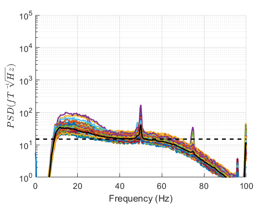
If you can spot any channels in the PSD that are behaving differently to other channels we can interactively identify them by clicking on the plot. We can then set the bad channels with the following code.
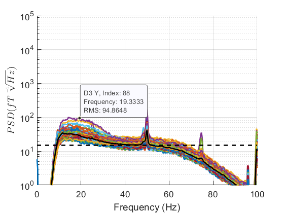
As all channels appear to be behaving fairly similarly we won’t mark any as bad but the code should you wish to do so is below.
Note
If you change an M/EEG object(D) you should call the save method to make your changes permanent.
Epoching and baseline correction
Now that we have modelled the interference in our data we can cut our data up into the time periods we are interested in. To do this we require that a trigger channel exists in our data set when some stimuli was presented to a participant. In this case we are interested in the 50ms before the stimuli up until 200ms after the stimuli. This time window is specified with the S.timewin argument. The channel that encodes when the stimuli is presented is channel Trigger 6 Z and we can specify this with the S.triggerChannels argument.
S =[];
S.D=mD;
S.timewin=[-50 200];
S.triggerChannels ={'Trigger 6 Z'};
eD= spm_opm_epoch_trigger(S);
S=[];
S.D = eD;
S.timewin = [-50 0];
eD = spm_eeg_bc(S);
Note
SPM automatically baseline corrects data that has a negative time window. if you do not have a negative time window you will need to do baseline correction separately( see spm_eeg_bc).
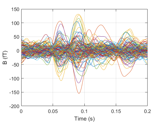
Averaging
We can now compute our evoked response by averaging across trials. The function spm_eeg_average has 1 key argument: S.D. We can then plot the average response for all channels.
S=[];
S.D=eD;
muD = spm_eeg_average(S);
MEGind = indchantype(eD,'MEGMAG');
used = setdiff(MEGind,badchannels(muD));
pl =muD(used,:,:)';
figure();
plot(muD.time(),pl)
xlabel('Time (s)')
ylabel('B (fT)')
grid on
ax = gca; % current axes
ax.FontSize = 13;
ax.TickLength = [0.02 0.02];
fig= gcf;
fig.Color=[1,1,1];
xlim([0,.250])
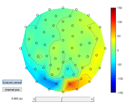
Topoplots
Displaying OPM topographies is non trivial for 2 reasons: 1. For small channel arrays 2D representations of 3D data may not look very good. 2. OPMs measure multiple components of the magnetic field at the same point in space and the sampled field pattern is not necessarily smooth.
As such for now we will only display the radial component of the magnetic field measurement(which is a smooth interpretable field). We can do this with spm_opm_plotScalpData and we will initially look at the peak around 70ms.
Note
If you think OPM scalp data should be displayed differently please open an issue on GitHub.
A complete script
Below we include the whole script required to reproduce the figures in this tutorial.
%- read data
%--------------------------------------------------------------------------
S = [];
S.data ='OPM_meg_001.cMEG';
S.positions= 'OPM_HelmConfig.tsv';
D = spm_opm_create(S);
%- PSD
%--------------------------------------------------------------------------
S=[];
S.triallength = 3000;
S.plot=1;
S.D=D;
S.channels='MEG';
spm_opm_psd(S);
ylim([1,1e5])
%- highpass
%--------------------------------------------------------------------------
S=[];
S.D=D;
S.freq=[10];
S.band = 'high';
fD = spm_eeg_ffilter(S);
%- lowpass
%--------------------------------------------------------------------------
S = [];
S.D = fD;
S.freq = [70];
S.band = 'low';
fD = spm_eeg_ffilter(S);
%- adaptive multipole models
%--------------------------------------------------------------------------
S = [];
S.D = fD;
S.corrLim = .98;
mD = spm_opm_amm(S);
%- psd
%--------------------------------------------------------------------------
S=[];
S.triallength = 3000;
S.plot=1;
S.D=mD;
S.channels='MEG';
[~,freq]=spm_opm_psd(S);
ylim([1,1e5])
%- epoch
%--------------------------------------------------------------------------
S =[];
S.D=mD;
S.timewin=[-50 200];
S.triggerChannels ={'Trigger 6 Z'};
eD= spm_opm_epoch_trigger(S);

S=[];
S.D = eD;
S.timewin = [-50 0];
eD = spm_eeg_bc(S);
%- average
%--------------------------------------------------------------------------
S=[];
S.D=eD;
muD = spm_eeg_average(S);
MEGind = indchantype(eD,'MEGMAG');
used = setdiff(MEGind,badchannels(muD));
pl =muD(used,:,:)';
figure();
plot(muD.time(),pl)
xlabel('Time (s)')
ylabel('B (fT)')
grid on
ax = gca; % current axes
ax.FontSize = 13;
ax.TickLength = [0.02 0.02];
fig= gcf;
fig.Color=[1,1,1];
xlim([0,.20])
%- topoplot
%--------------------------------------------------------------------------
S=[];
S.D = muD;
S.T=.066
spm_opm_plotScalpData(S);
caxis([-150, 150])