EEG Mismatch negativity data
This chapter describes the analysis of a 128-channel single subject EEG data set acquired from a study of mismatch negativity in the auditory system (Garrido et al. 2008). We thank Marta Garrido for providing us with these data. The experiment comprised an auditory oddball paradigm in which subjects heard standard (500Hz) and deviant (550Hz) tones, occurring 80% (480 trials) and 20% (120 trials) of the time, respectively, in a pseudo-random sequence subject to the constraint that two deviant tones did not occur together.
EEG data were recorded with a Biosemi1 system at 128 scalp electrodes
and a sampling rate of 512Hz. Vertical and horizontal eye movements were
monitored using EOG electrodes. See (Garrido et al. 2008) for full
details of experimental stimuli and recording. To proceed with the data
analysis, first download the data set from the SPM website2. The data
comprises a file called subject1.bdf whose size is roughly 200MB. We
will refer to the directory in which you have placed it as DATA_DIR.
This chapter takes you through different stages of analysis:
-
Preprocessing
-
Sensor space analysis
-
Source reconstruction
-
Dynamic Causal Modelling
Preprocessing
Unlike preprocessing in SPM8 which consisted of a sequence of steps
applied to a dataset using the GUI, preprocessing in SPM12 is most
conveniently done by building and configuring a batch pipeline and then
running it. The advantage of that is that a batch pipeline can
immediately be applied to another dataset with perhaps minor
adjustments. It is also possible to call preprocessing functions from
more low-level scripts. These scripts can be generated from the history
feature of SPM, saved in preprocessed datasets and then modified. There
is also an example MATLAB script under
man\(\backslash\)example_scripts\(\backslash\)history_subject1.m in
the SPM distribution which repeats the preprocessing route we take here.
Simple conversion and reviewing
At the MATLAB prompt type spm eeg, from the
Convert dropdown menu select
Convert. Select the subject1.bdf file
and press "Done". At the prompt “Define settings?” select “just read”.
SPM will now read the original Biosemi format file and create an SPM
compatible data file, called spmeeg_subject1.mat and
spmeeg_subject1.dat in the directory containing the original data file
(DATA_DIR). From "Display" dropdown menu select "M/EEG". In the
file selection dialogue that comes up select spmeeg_subject1.mat and
press "Done". The file will now be opened in the SPM reviewing tool.
By default the tool will be opened on the ‘history’ tab that shows the
sequence of preprocessing steps applied to the dataset until now (in
this case there is just a single line for ‘Conversion’). You can switch
to ‘channels’ and ‘trials’ tabs to see the list of channels and events
in the dataset. Then switch to ‘EEG’ tab to review the continuous data.
Note that due to large DC shifts in this particular dataset all the
channels initially look flat and it is necessary to zoom in to actually
see the EEG traces.
Preparing batch inputs
Press the ‘Prepare SPM file’ button in the top right corner of the reviewing tool window. A menu will appear in the SPM interactive window (the small window usually located at the bottom left). Note that on the latest version of MacOS the menu might appear in the menu bar at the top when clicking on the interactive window and not in the window itself. Similar functionality can also be accessed without the reviewing tool by choosing Prepare from the Convert dropdown menu. Here we will prepare in advance some inputs that will be necessary for the subsequent preprocessing stages. The reason this needs to be done is that all inputs to the batch tool must be provided in advance before hitting the ‘Run’ button. Some processing steps (e.g. channel selection) are much easier to do interactively, first SPM will read some information from the dataset (e.g. list of all channels) and then ask the user to make a choice using GUI. For these steps interactive GUI tools have been added to the ‘Prepare’ interface under ‘Batch inputs’ menu. These tools save the result of the user’s choice in a MAT-file that can be provided as input to batch. Usually it should be sufficient to perform the interactive steps for one dataset and the results can be used for all datasets recorded in the same way. So although preparing something in advance and only using it later may seem cumbersome at first, the idea is to facilitate batch processing of multiple datasets which is what most people routinely do. As the first step we will make a list of channels to be read. The original files contains some unused channels that do not need to be converted and we can exclude them from the beginning. From ‘Batch inputs’ menu select ‘Channel selection’. A popup window will appear with the list of all channels in the dataset. A subset of channels can be selected (use Shift- and Ctrl- clicks if necessary to select multiple items). Select all EEG channels (these are the channels from A1 to D32). In addition select 3 channels that were used in the experiment to record EOG: EXG1, EXG2 and EXG3. Press ‘OK’ and save the selection as a MAT-file named e.g ‘channelselection.mat’.
Next we will prepare an input for the Montage step. This step will derive vertical and horizontal EOG channels by subtracting pairs of channels located above and below the eye and below and lateral to the eye respectively. It will also change the recording reference to be the average of all EEG channels. There are several ways to create montage specifications: using script, GUI, batch and even copying and pasting from Excel. Here we will show the steps to create the montage solely using the GUI, which for this particular dataset requires several steps. First we will change the channel type of the channels containing EOG. Select ‘EOG’ from the ‘Channel types’ menu and in the channel list that comes up select EXG1, EXG2 and EXG3 channels and press OK. Next from ‘Batch inputs’ menu select ‘Montage’ and there select ‘Re-reference’. In the channel list that comes up press ‘Select all’, press OK and save the montage e.g. as ‘avref.mat’. This montage subtracts the average of all channels from each channel - this is called ‘conversion to average reference’. We would now like to add to the montage two extra lines deriving the EOG channels. To do that from the same ‘Montage’ submenu select ‘Custom montage’ and in the window that appears press ‘Load file’ and load the previously saved ‘avref.mat’. Click on the button at the top left of the montage table to select the whole table and press Ctrl-C (or equivalent on your system). Now press ‘OK’ , open ‘Custom montage’ tool again press the top left button again and press Ctrl-V (or equivalent). On some systems instead of pressing Ctrl-C and Ctrl-V it is better to select ‘Copy’ and ‘Paste’ respectively after right-clicking the corner button. Now scroll to the bottom of the table. On line 129 write ‘HEOG’ instead of ‘EXG1’. On line 130 write ‘VEOG’ instead of ‘EXG2’. Click to select the whole of line 131 and press ‘Delete’ (or equivalent). Finally scroll to the bottom right of the table and add ‘-1’ in line 129 in the column for ‘EXG2’ . Also add ‘-1’ in line 130 in the column for ‘EXG3’. This defines the HEOG channel as the difference of EXG1 and EXG2 and VEOG as the difference of EXG2 and EXG3. Save the montage by pressing the ‘Save as’ button and naming the file ‘avref_eog.mat’. Press ‘OK’ to close the ‘Custom montage’ tool.
An alternative way for creating a montage specification is using a short
script available in the example_scripts folder: montage_subject1.m.
You are welcome to try it by copying this script into DATA_DIR and
running it. This will generate a file named MONT_EXP.mat.
The final input we should prepare in advance is trial definition for
epoching. Select ‘Trial definition’ from ‘Batch inputs’ menu. Choose the
peri-stimulus time window as -100 400. Choose 2 conditions. You can
call the first condition “standard”. A GUI pops up which gives you a
complete list of all events in the EEG file. The standard condition had
480 trials, so select the type with value 1 and press OK. Leave ‘Shift
triggers’ at default 0. The second condition can be called “rare”. The
rare stimulus was given 120 times and has value 3 in the list. Select
this trial type and press OK. Leave ‘Shift triggers’ at default 0.
Answer”no” to the question “review individual trials”, and save the
trial definition as trialdef.mat.
Preprocessing step by step
We will now build a complete batch pipeline for preprocessing and statistical analysis of the MMN dataset. We will start with running different steps one-by-one and then show how to chain these steps to run them all together.
Convert
As the first step we will repeat the data conversion, this time using
batch. This makes it possible to refine the conversion settings and make
conversion part of the complete preprocessing pipeline that can be
reused later. Select Convert from the
Convert dropdown menu, select the
subject1.bdf file and this time answer ‘yes’ to ‘Define settings?’.
The conversion batch tool will appear. If you are not familiar with SPM
batch, the tool presents the configuration structure as a tree where you
can enter values and select different options from a list. For many
options there are default settings. Options where user input must be
provided are marked by the \(\leftarrow X\) sign on the right of the batch
window. All these entries must be specified to enable the ‘Run’ button
(green triangle at the toolbar) and run the batch. In our case we will
provide the raw dataset name and channel selection. Click on ‘Channel
selection’ and in the list of option appearing below the configuration
tree display click on ‘Delete: All(1)’. This will remove the default
setting of selecting all channels. Then click on ‘New: Channel file’. An
entry for ‘Channel file’ will appear under ‘Channel selection’.
Double-click on it and select the previously saved
channelselection.mat file. The ‘Run’ button is now enabled. Press on
it to run the batch and convert the dataset.
Montage
Select Montage from the
Preprocessing dropdown menu. Montage
batch tool will appear. Double-click on ‘File name’ and select the
spmeeg_subject1.mat file created by conversion. Click on ‘Montage file
name’ and select the avref_eog.mat (or MONT_EXP.mat) file generated
as described above. Run the batch. The progress bar appears and SPM will
generate two new files Mspmeeg_subject1.mat and
Mspmeeg_subject1.dat.
Prepare
The previous step also assigned default locations to the sensors, as
this information is not contained in the original Biosemi *.bdf file.
It is usually the responsibility of the user to link the data to sensors
which are located in a coordinate system. In our experience this is a
critical step. Here we will perform this step using ‘Prepare’ batch.
Select Prepare (batch) from the
Convert dropdown menu. Select
Mspmeeg_subject1.mat dataset as input. Click on ‘Select task(s)’ and
from the options list select ‘New: Load EEG sensors’. Under ‘Select EEG
sensors file’ select sensors.pol file provided with the example
dataset and run the batch. At this step no new files will be generated
but the same dataset will be updated.
High-pass filter
Filtering the data in time removes unwanted frequency bands from the
data. Usually, for evoked response analysis, the low frequencies are
kept, while the high frequencies are assumed to carry noise. Here, we
will use a highpass filter to remove ultra-low frequencies close to DC,
and a lowpass filter to remove high frequencies. We filter prior to
downsampling because otherwise high-amplitude baseline shifts present in
the data will generate filtering artefacts at the edges of the file.
Select Filter from the
Preprocessing dropdown menu. Select
Mspmeeg_subject1.mat dataset as input. Click on ‘Band’ and choose
‘Highpass’. Double-click on ‘Cutoff(s)’ and enter 0.1 as the cutoff
frequency. Run the batch. The progress bar will appear and the resulting
filtered data will be saved in files fMspmeeg_subject1.mat and
fMspmeeg_subject1.dat.
Downsample
Here, we will downsample the data in time. This is useful when the data
were acquired like ours with a high sampling rate of 512 Hz. This is an
unnecessarily high sampling rate for a simple evoked response analysis,
and we will now decrease the sampling rate to 200 Hz, thereby reducing
the file size by more than half. Select
Downsample from the
Preprocessing dropdown menu and select
the fMspmeeg_subject1.mat file. Choose a new sampling rate of 200
(Hz). The progress bar will appear and the resulting data will be saved
to files dfMspmeeg_subject1.mat and dfMspmeeg_subject1.dat.
Low-pass filter
Select Filter from the
Preprocessing dropdown menu. Select
dfMspmeeg_subject1.mat dataset as input. Keep the band at default
‘Lowpass’. Double-click on ‘Cutoff(s)’ and enter 30 as the cutoff
frequency. Run the batch. The progress bar will appear and the resulting
filtered data will be saved in files fdfMspmeeg_subject1.mat and
fdfMspmeeg_subject1.dat.
Epoch
Here we will epoch the data using the previously created trial
definition file. Note that it is possible to create a trial definition
file based on one dataset and use it on a different dataset as long as
events are coded the same way in both datasets Select
Epoch from the
Preprocessing dropdown menu. Select the
fdfMspmeeg_subject1.mat file as input. For ‘How to define trials’
select ‘Trial definition file’ and choose the previously saved
‘trialdef.mat’. The progress bar will appear and the epoched data will
be saved to files efdfMspmeeg_subject1.mat and
efdfMspmeeg_subject1.dat.
Artefacts
A number of different methods of artefact removal are implemented in SPM. Here, we will demonstrate a simple thresholding method. However, before doing so, we will look at the data in the display:
-
Choose “M/EEG” from the “Display” dropdown menu.
-
Select the
efdfMspmeeg_subject1.matfile. -
Click on the “EEG” tab.
-
Press the “scalp” radio button.
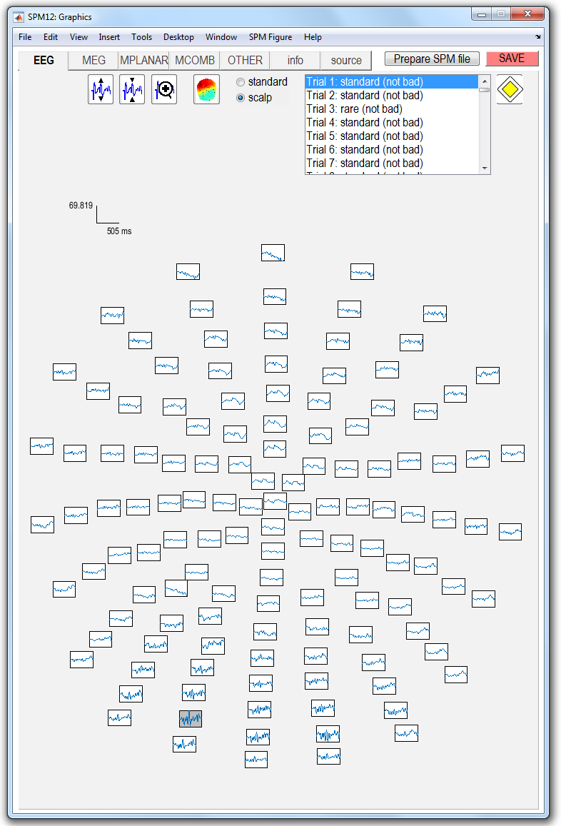
The time-series for the first trial will then appear in the topographical layout shown in Figure 1.1.
You will see that Channel 14, second-row from bottom, left hemisphere, contains (slightly) higher variability data than the others . Right-click on the channel; this tells you that this channel is “A14”. You will also see as an entry in this menu “bad: 0”. Select this entry, and click the left button. This will make the menu disappear, but the channel now has a grey background. You have marked this channel as bad. Click on “save”in the top-right corner. This channel will then be ignored in subsequent processing. In fact this channel probably doesn’t need removing, but we do so for teaching purposes only.
Select Detect artefacts from the
Preprocessing dropdown menu. Select the
efdfMspmeeg_subject1.mat file as input. Double click “How to look for
artefacts” and a new branch will appear. It is possible to define
several sets of channels to scan and several different methods for
artefact detection. We will use simple thresholding applied to all
channels. Click on “Detection algorithm” and select “Threshold channels”
in the small window below. Double click on “Threshold” and enter 80 (in
this case \(\mu V\)). The batch is now fully configured. Run it by
pressing the green button at the top of the batch window.
This will detect trials in which the signal recorded at any of the channels exceeds 80 microvolts (relative to pre-stimulus baseline). These trials will be marked as artefacts. Most of these artefacts occur on the VEOG channel, and reflect blinks during the critical time window. The procedure will also detect channels in which there are a large number of artefacts (which may reflect problems specific to those electrodes, allowing them to be removed from subsequent analyses).
For our dataset, the MATLAB window will show:
81 rejected trials: 3    4    5    7   26   27   28    [...]
1 bad channels: A14
Done    'M/EEG Artefact detection'
A new file will also be created, aefdfMspmeeg_subject1.mat.
As an alternative to the automatic artefact rejection tool, you can also
look at the interactive artefact removal routines available from
Toolbox \(\rightarrow\) MEEG tools \(\rightarrow\)
Fieldtrip visual artifact rejection.
Averaging
To produce an ERP, select Average from
the Average dropdown menu and select the
aefdfMspmeeg_subject1.mat file as input. At this point you can perform
either ordinary averaging or “robust averaging”. Robust averaging makes
it possible to suppress artefacts automatically without rejecting trials
or channels completely, but just the contaminated parts. For robust
averaging select ‘Robust’ under ‘Averaging type’. Also select “yes” for
“Compute weights by condition” 3. After running the batch a new
dataset will be generated maefdfMspmeeg_subject1.mat. This completes
the preprocessing steps.
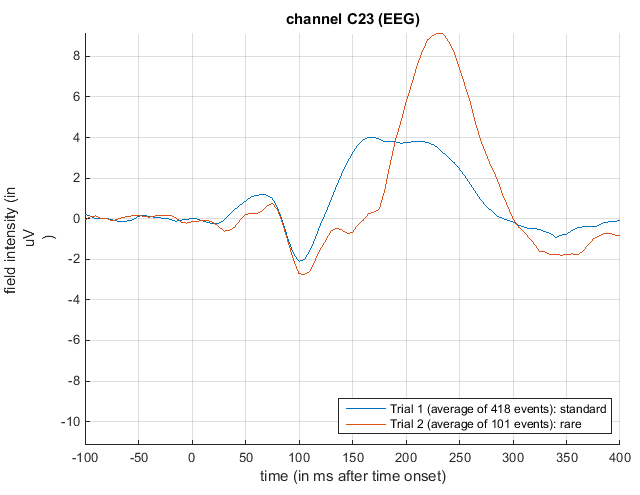
Open the averaged dataset in the reviewing tool. To look at the ERP, click on the EEG tab, and press the “scalp” radio button. Now hold the Shift button down on the keyboard whilst selecting trial 2 with the left mouse button in the upper right corner of the graphics window. This will overlay responses to standard and rare trials on the same figure axes.
Now press the “plus” icon at the top of this graphics window and select channel C23 (seventh central channel down from the top) with a left mouse click. This will plot the ERPs shown in Figure 1.2.
Automatisation of preprocessing
The preprocessing steps we performed separately for instructive purposes can all be run together as part of a pipeline. Once specified such a pipeline can be reused on a different input dataset from a different session or subject. There are two ways to build a pipeline in SPM. One way is to use the batch tool as we did above but instead of configuring and running each step separately to configure all the steps as a chain and run them together. The second way is to use a script calling the low-level preprocessing functions. Such a script can be generated semi-automatically from the history of a pre-processed file. For more complicated pipelines there can be scripts that configure and run batch pipelines for some steps with some processing with the user’s own code in between. For different tools available in SPM the ‘division of labour’ between the code that is part of the batch tools and more low-level code can be different. For M/EEG preprocessing running low-level functions without the batch is quite simple whereas for statistics or source reconstruction it is much easier to use the batch code. Some examples will be provided below.
Building a batch pipeline
Press the ‘Batch’ button at the bottom right of the SPM menu window. An empty batch tool will be open. Processing steps can now be added via the menu. From the SPM menu in the batch window select M/EEG submenu and in the submenu select ‘Conversion’. The conversion configuration tree will appear. Configure it as described above (the ‘Conversion’ section). Now without running the batch or closing the batch window go back to the M/EEG submenu and select the ‘Preprocessing’ sub-submenu and from there ‘Montage’. On the left of the batch window ‘Montage’ will appear in module list. Click on it to switch to the montage configuration interface. Now comes the critical difference from the previously described step-by-step processing. Single-click on ‘File name’. The ‘Dependency’ button will appear at the bottom right part of the batch window. Press this button. A list will appear with the outputs of all the previous batch modules. In our case there is only one item in the list - the output of conversion. Select it and press ‘OK’. The rest of montage configuration is as described in the ‘Montage’ section above. Now continue with ‘Prepare’ and the other modules in similar fashion. Once batch is fully configured it can be run by pressing the green triangle button.
Note that you can use “Delete” batch tool from the “Other” submenu to
delete the intermediate datasets that you don’t need once the final
processing step has been completed. Finally, you can save the full batch
pipeline as MATLAB code. To do that select “Save batch” from the “File”
menu of the batch tool. At the bottom of the dialogue box that appears,
select “MATLAB .m script file”. Save the batch as e.g. mmnbatch.m. You
can then open the batch .m file either in the batch tool to reproduce
the configured pipeline or in the MATLAB editor. The generated MATLAB
code is quite straightforward to interpret. It basically creates a data
structure closely corresponding to the structure of the configuration
tree in the batch tool. The structure can be easily modified e.g. by
replacing one input dataset name with another. Things one should be
careful about include not changing the kind of brackets around different
variables, and also paying attention to whether a list is a row or
column cell array of strings. Once the matlabbatch structure is
created by the code in a batch m-file (or loaded from a batch mat-file)
it can immediately be run from a script without the need to load it in a
batch GUI. Assuming that the batch structure is called matlabbatch,
the command for running it is spm_jobman(’run’, matlabbatch).
Generating scripts from history
The evoked response file (and every other SPM MEEG data file) contains a history-entry which stores all of the above preprocessing steps. You can take this history and produce a script that will re-run the same analysis which you entered using the GUI. See the “history” tab in the “info” section when displaying the data. Chapter [Chap:eeg:preprocessing] provides more details on this.
Sensor space analysis
A useful feature of SPM is the ability to use Random Field Theory to correct for multiple statistical comparisons across N-dimensional spaces. For example, a 2D space representing the scalp data can be constructed by flattening the sensor locations and interpolating between them to create an image of MxM pixels (when M is user-specified, eg M=32). This would allow one to identify locations where, for example, the ERP amplitude in two conditions at a given timepoint differed reliably across subjects, having corrected for the multiple t-tests performed across pixels. That correction uses Random Field Theory, which takes into account the spatial correlation across pixels (i.e, that the tests are not independent). Here, we will consider a 3D example, where the third dimension is time, and test across trials within this single subject. We first create a 3D image for each trial of the two types, with dimensions M\(\times\)M\(\times\)S, where S=101 is the number of samples (time points). We then take these images into an unpaired t-test across trials (in a 2nd-level model) to compare “standard” and “rare” events. We can then use classical SPM to identify locations in space and time in which a reliable difference occurs, correcting across the multiple comparisons entailed. This would be appropriate if, for example, we had no a priori knowledge where or when the difference between standard and rare trials would emerge. The appropriate images are created as follows.
Select ‘Convert to images’ from the ‘Images’ dropdown menu. In the batch
tool that will appear select the aefdfMspmeeg_subject1.mat as input.
For the ‘Mode’ option select ‘scalp x time’. In the ‘Channel selection’
option delete the default choice (‘All’) and choose ‘Select channels by
type’ with ‘EEG’ as the type selection. You can now run the batch.
SPM will take some time as it writes out a NIfTI image for each
condition in a new directory called aefdfMspmeeg_subject1. In our case
there will be two files , called condition_rare and
condition_standard. These are 4D files, meaning that each file
contains multiple 3D scalp x time images, corresponding to non-rejected
trials. You can press “Display: images” to view one of these images.
Change the number in the ‘Frames’ box to select a particular trial
(first trial is the default). The image will have dimensions
32\(\times\)32\(\times\)101.
To perform statistical inference on these images:
-
Create a new directory, eg.
mkdir XYTstats. -
Press the “Specify 2nd level” button.
-
Select “two-sample t-test” (unpaired t-test)
-
Define the images for “Group 1” as all those in the file
condition_standard. To do that write ‘standard’ in the ‘Filter’ box and ‘Inf’ in the ‘Frames’ box of the file selector. All the frames will be shown. Right click on any of the frames in the list and choose ‘Select all’. Similarly for “Group 2” select the images fromcondition_rarefile. -
Finally, specify the new
XYTstatsdirectory as the output directory. -
Press the “save” icon, top left, and save this design specification as
mmn_design.matand press “save”. -
Press the green “Run” button to execute the job4 This will produce the design matrix for a two-sample t-test.
-
Now press “Estimate” in SPMs main window, and select the
SPM.matfile from theXYTstatsdirectory.
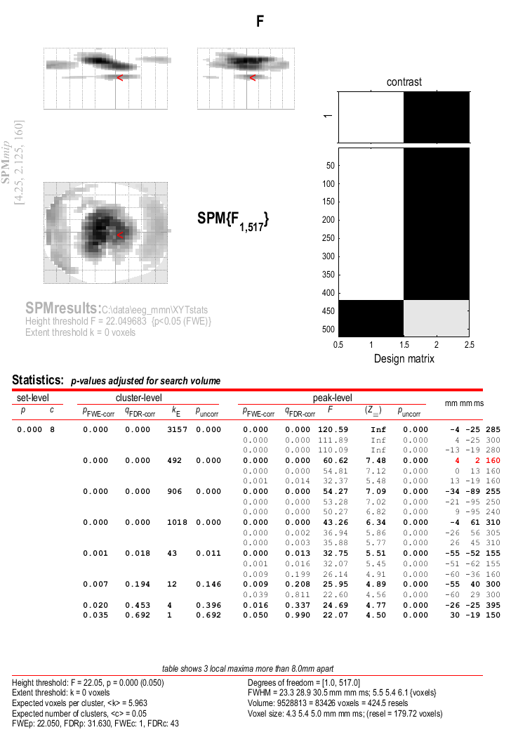
Now press “Results” and define a new F-contrast as [1 -1] (for help with these basic SPM functions, see eg. chapter [Chap:data:auditory]). Keep the default contrast options, but threshold at \(p<.05\) FWE corrected for the whole search volume and select “Scalp-Time” for the “Data Type”. Then press “whole brain”, and the Graphics window should now look like that in Figure 1.3. This reveals a large fronto-central region within the 2D sensor space and within the time epoch in which standard and rare trials differ reliably, having corrected for multiple F-tests across pixels/time. An F-test is used because the sign of the difference reflects the polarity of the ERP difference, which is not of primary interest.
The cursor in Figure 1.3 has been positioned by selecting the second cluster in the results table. This occurs at time point 160ms post stimulus.
Now:
-
Press the right mouse button in the MIP
-
Select “display/hide channels”
-
Select the
maefdfMspmeeg_subject1.matfile.
This links the SPM.mat file with the M/EEG file from which the EEG
images were created. It is now possible to superimpose the channel
labels onto the spatial SPM, and also to “goto the nearest channel”
(using options provided after a right mouse click, when navigating the
MIP).
We have demonstrated sensor space analysis for single-subject data. More frequently, one would compute ERP images for each subject, smooth them, and then perform paired t-tests over subjects to look for condition differences. See (Garrido et al. 2008) for a group analysis of MMN data.
Finally, if one had more constrained a priori knowledge about where and when the differences would appear, one could perform a Small Volume Correction (SVC) based on, for example, a box around fronto-central channels and between 100 and 200ms poststimulus. We also refer the reader to chapter [Chap:eeg:sensoranalysis] for further details on sensor space analysis.
Batching statistics
The above described steps can be automatised using the batch tool. The relevant modules can be found in the ‘Stats’ submenu of the ‘SPM’ menu. They are ‘Factorial design specification’, ‘Model estimation’, ‘Contrast manager’ and ‘Results report’. We will not go over the batch steps in detail but you should be able to build the batch now based on previously described principles. One point worth mentioning is that preprocessing and statistics can be done in a single batch with dependencies. For that the ‘Convert2Images’ module can be added to the batch twice and the ‘Conditions’ option in this module can be used to convert the ‘standard’ and ‘rare’ conditions separately in the two instances of the module to match the two separate dependencies from ‘Factorial design specification’.
Source reconstruction
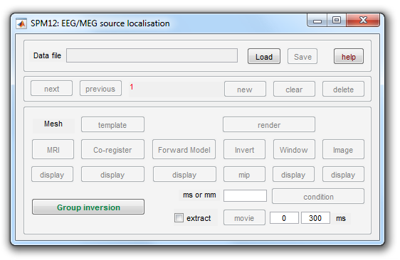
Source reconstruction comprises forward modeling and inverse modeling steps and is implemented by pressing the 3D source reconstruction button in SPM’s top-left window. This brings up the source localisation GUI shown in Figure 1.4. The following subsections detail each of the steps in a source reconstruction analysis. We also advise the reader to consult the reference material in chapter [Chap:eeg:imaging].
Mesh
The first step is to load the data and create a cortical mesh upon which M/EEG data will be projected:
-
Press the “Load” button in the source localisation GUI and select the file
maefdfMspmeeg_subject1.mat. -
Enter “Standard” under “Comment/Label for this analysis” and press OK.
-
Now press the “template” button.
-
For “Cortical mesh”, select “normal”.
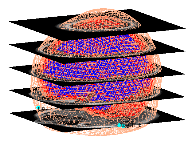
SPM will then form the “standard” or “canonical” cortical mesh shown in the Graphics window which, after rotation, should look like Figure 1.5
Coregister
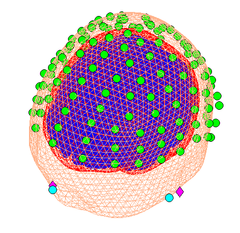
Now press the “Co-register” button. This will create further output in the Graphics window, the upper panel of which should like like Figure 1.6.
In this coregister step we were not required to enter any further parameters. However, if you are not using the template (or “canonical” mesh) or if at the “prepare” stage above you loaded your own (non-standard) sensor positions then you will be asked for the locations in MNI coordinates of the fiducial positions.
Forward model
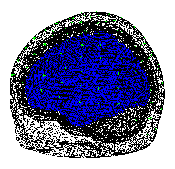
Now press the “Forward model” button. Then select “EEG-BEM” in response
to the “Which EEG head model?” question. SPM will then use a Boundary
Element Method (BEM) which will take a few minutes to run. Upon
completion SPM will write the single_subj_T1_EEG_BEM.mat file into the
canonical subdirectory of your SPM distribution. The Graphics window
should now appear as in
Figure 1.7.
The next time you wish to use an EEG-BEM solution based on the template
mesh, SPM will simply use the date from the single_subj_T1_EEG_BEM.mat
file (so this step will be much quicker the next time you do it). The
same principle applies to EEG-BEM solutions computed from meshes based
on subjects individual MRIs.
Invert
Now press the Invert button and
-
Select an “Imaging” reconstruction.
-
Select “Yes” for “All conditions or trials”.
-
Select “Standard” for Model.
SPM will now compute a leadfield matrix and save it in the file
SPMgainmatrix_maefdfMspmeeg_subject1.mat placed in DATA_DIR. This
file can be replaced with one computed using other methods for computing
the lead field (e.g. methods external to SPM). The forward model will
then be inverted using the Multiple Sparse Priors (MSP) algorithm (the
progress of which is outputted to the MATLAB command window). SPM will
produce, in the Graphics window, (i) a Maximum Intensity Projection
(MIP) of activity in source space (lower panel) and (ii) a time series
of activity for (upper panel) each condition.
The “ms or mm” window has three functionalities (i) if you enter a single number this will be interpreted as ms, (ii) if you enter two numbers this will be interpreted as a time window for plotting movies (see below), (iii) if you enter 3 numbers this will be interpreted as MNI coordinates for a time series plot.
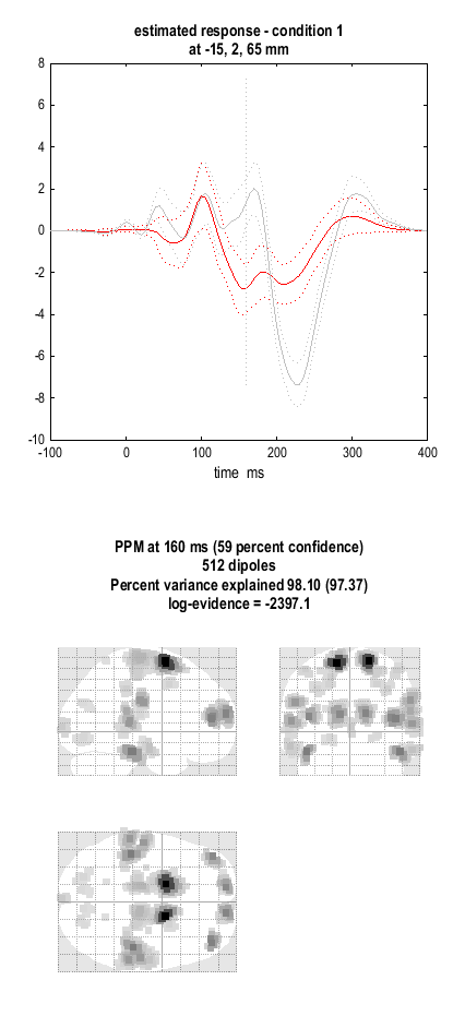
Now enter “160” for “ms or mm” and press the MIP button, to see a MIP of activity in source space at 160ms post-stimulus, and the time series of activities (top panel) at the position with largest magnitude signal. The corresponding graphic is shown in Figure 1.8. By toggling the “Condition” button, and pressing MIP each time, you can view the spatial distribution of activity for the different conditions (at the selected time point).
Batching source reconstruction
All the functionality of source reconstruction can be batched, using the tools from ‘Source reconstruction’ submenu of ‘M/EEG’. ‘Head model specification tool’ performs mesh generation, coregistration and forward model specification. ‘Source inversion’ tool computes the inverse solution and ‘Inversion results’ tool summarises the inversion results as images. One tip when incorporating source reconstruction batch in a script is one should be aware that the batch reads the @meeg object from disk and saves the results to disk but does not update the @meeg object in the workspace. Thus, it is advised to save any changes to the object before running the batch (D.save) and to reload the object after running the batch (D = D.reload).
Dynamic Causal Modeling
Many of the functionalities of DCM for M/EEG are described in more detail in the reference chapter [Chap:eeg:DCM]. In this chapter we demonstrate only the “DCM for ERP” model. Users are strongly encouraged to read the accompanying theoretical papers (David et al. 2006; Kiebel, David, and Friston 2006). Briefly, DCM for ERP fits a neural network model to M/EEG data, in which activity in source regions is described using differential equations based on neural mass models. Activity in each region comprises three populations of cells; pyramidal, local excitatory and local inhibitory. Fitting the model will then allow you to plot estimated activity in each cell population in each region. It will also provide estimates of the long range connections between regions, and show how these values are changed by experimental manipulation (eg. rare versus standard trial types).
In the example_scripts folder of the SPM distribution, we also provide
an example script that will run a DCM-for-ERP analysis of this data.
This can be edited to implement your own analysis.
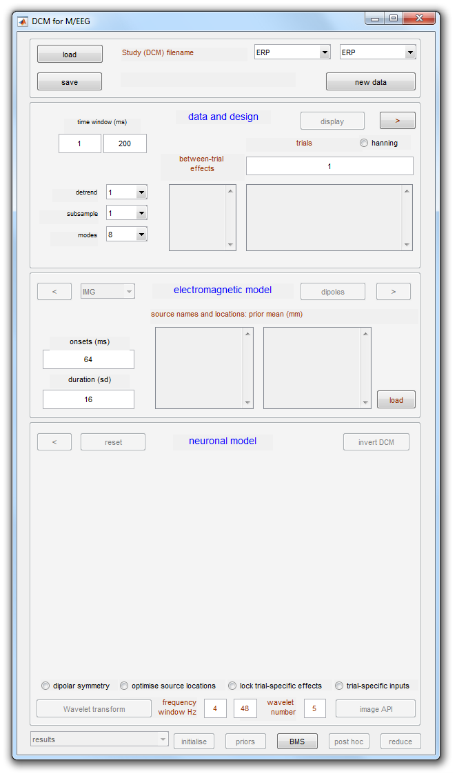
Pressing the “DCM” button will open up the DCM GUI shown in Figure 1.9.
(a)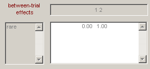 (b)
(b)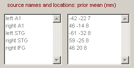 (c)
(c)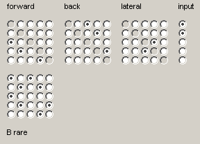
We will now complete the three model specification entries shown in Figure 1.10:
-
Press the “new data” button and select the
maefdfMspmeeg_subject1.matfile. -
Enter the “between-trial effects” and design matrix information shown in Figure 1.10(a).
-
Press the “Display” button.
This completes the data specification stage. Now:
-
Press the right hand arrow to move on to the specification of the electromagnetic model.
-
Instead of “IMG” select “ECD” for the spatial characteristics of the sources.
-
Now enter the names and (prior mean) locations of the sources shown in Figure 1.10(b).
-
Pressing the “dipoles” button will create an interactive display in the graphics window showing the prior source positions.
This completes the specification of the electromagnetic model. Now:
-
Press the right hand arrow (next to the dipoles button) to move on to specification of the neuronal model.
-
Highlight the connectivity matrix radio buttons so that they correspond to those shown in Figure 1.10(c).
-
Press the (top left) ‘save’ button and accept the default file name.
-
Press ‘Invert DCM’
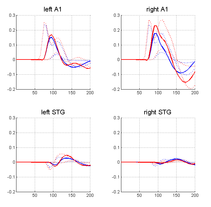
SPM will plot the progress of the model estimation in the MATLAB command window. Plots of data and the progressing model fit will be shown in SPM’s graphics window. The algorithm should converge after five to ten minutes (in 64 iterations). Now select the “ERPs (sources)” option from the pull down menu to the right of the “Estimated” button. This will produce the plot shown in Figure 1.11. The values of the connections between areas can be outputted by selecting eg “Coupling(A)” from the pull-down menu in the DCM GUI. This will allow you to interrogate the posterior distribution of model parameters. It is also possible to fit multiple models, eg. with different numbers of regions and different structures, and to compare them using Bayesian Model Comparison. This is implemented by pressing the BMS button (bottom right hand corner of the DCM window).
-
BioSemi: http://www.biosemi.com/ ↩
-
EEG MMN dataset: http://www.fil.ion.ucl.ac.uk/spm/data/eeg_mmn/ ↩
-
In this case we do not want to pool both conditions together because the number of standard and rare trials are quite different. ↩
-
Note that we can use the default “nonsphericity” selections, i.e, that the two trial-types may have different variances, but are uncorrelated. ↩