fMRI analysis 
Only the main characteristics of the fMRI analysis are described below; for a more detailed demonstration of fMRI analysis, read previous tutorial chapters describing fMRI analyses.
Toggle the modality from EEG to fMRI, and change directory to the fMRI subdirectory (either in MATLAB, or via the “CD” option in the SPM “Utils” menu)
Preprocessing the fMRI data
Press the Batch button and then:
-
Select Spatial: Realign: Estimate & Reslice from the SPM menu, create two sessions, and select the 390
fM*.imgEPI images within the corresponding Session1 / Session 2 subdirectories (you can use the filter^fM.*). In the “Resliced images” option, choose “Mean Image Only”. -
Add a Spatial: Coreg: Estimate module, and select the
smri.imgimage in thesMRIdirectory for the “Reference Image” and select a “Dependency” for the “Source Image”, which is the Mean image produced by the previous Realign module. For the “Other Images”, select a “Dependency” which are the realigned images (two sessions) from Realign. -
Add a Spatial: Segment module, and select the
smri.imgimage as the “Data”. -
Add a Spatial: Normalise: Write module, make a “New: Subject”, and for the “Parameter File”, select a “Dependency” of the “Deformation Field Subj-\(>\)MNI” (from the prior segmentation module). For the “Images to Write”, select a “Dependency” of the “Coreg: Estimate: Coregistered Images” (which will be all the coregistered EPI images) and “Segment: INU corrected” (which will be the intensity nonuniformity corrected structural image). Also, change the “Voxel sizes” to [3 3 3], to save diskspace.
-
Add a Spatial: Smooth module, and for “Images to Smooth”, select a “Dependency” of “Normalise: Write: Normalised Images (Subj 1)”.
-
Save the batch file (e.g, as
batch_fmri_preproc.mat, and then press the “Run” button.
These steps will take a while, and SPM will output some postscript files
with the movement parameters and the coregistration results (see earlier
chapters for further explanation). The result will be a series of 2 sets
of 390 swf*.img files that will be the data for the following
1st-level fMRI timeseries analysis.
Statistical analysis of fMRI data
First make a new directory for the stats output, e.g, a Stats
subdirectory within the fMRI directory.
Press the batch button and then:
-
Select “Stats: fMRI model specification” from the SPM module menu, and select the new
Statssubdirectory as the “Directory”. -
Select “Scans” for “Units of design”.
-
Enter
2for the “Interscan interval” (i.e, a 2s TR). -
Create a new session from the “Data & Design” menu. For “Scans”, select all the
swf*.imgfiles from theSession1subdirectory (except the mean). Under “Multiple Conditions”, click “Select File”, and select thetrials_ses1.matfile that is provided with these data. (This file just contains the onsets, durations and names of every event within each session.). For “Multiple regressors”, click “Select File”, and select therp*.txtfile that is also in theSession1subdirectory (created during realignment). -
Repeat the above steps for the second session.
-
Under “Basis Functions”, “Canonical HRF” add the “Time and Dispersion” derivatives.
-
Then add a “Stats: Model estimation” module, and for the “Select SPM.mat”, choose the “Dependency” of the
SPM.matfile from the previous “fMRI model specification” module. -
Add a “Stats: Contrast Manager” module, and for the “Select SPM.mat”, choose the “Dependency” of the
SPM.matfile from the previous “Model Estimation module”. -
Under “Contrast Sessions”, create a new F-contrast with a “Name” like
faces vs scrambled (all BFs)and then enter[eye(3) -eye(3) zeros(3,6)]. This will produce a 3x12 matrix that picks out the three basis functions per condition (each as a separate row), summing across the two conditions (with zeros for the movement parameter regressors, which are of no interest). Then select “Replicate (average over sessions)”. -
Under “Contrast Sessions”, create a new F-contrast with a “Name” like
faces + scrambled vs Baseline (all BFs)and then enter the[eye(3) eye(3) zeros(3,6)]. Again, select “Replicate (average over sessions)”. -
Save the batch file (e.g, as
batch_fmri_stats.mat, and then press the “Run” button.
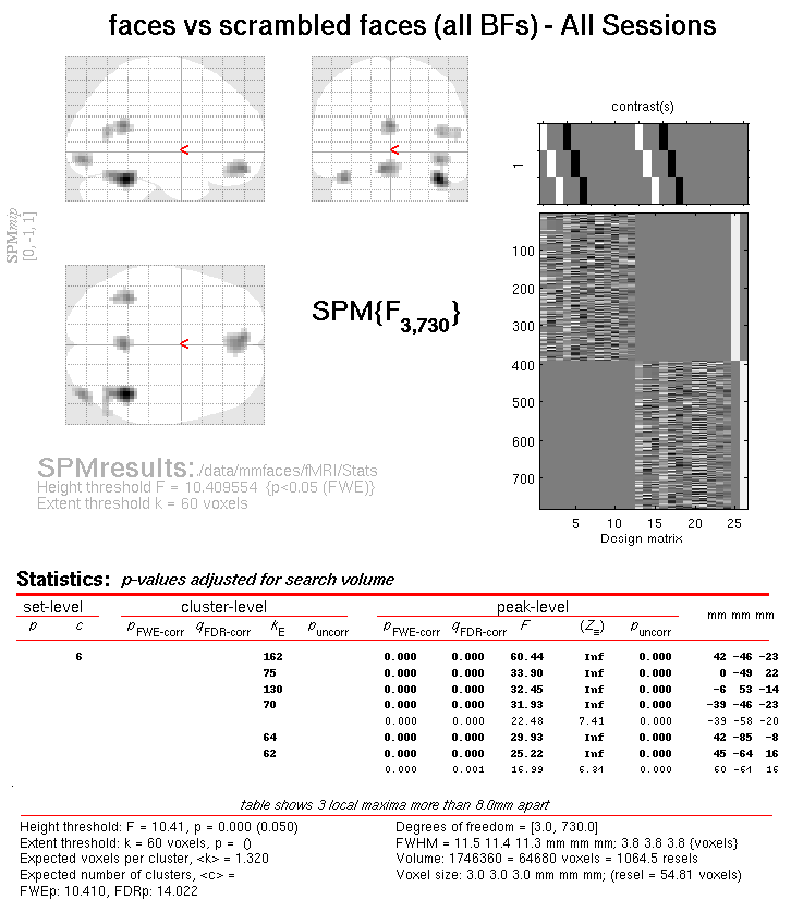
When this has finished, press Results and
select the SPM.mat file that should have been created in the new
Stats directory. The Contrast Manager window will appear, and you can
select the “faces vs scrambled (all BFs)” contrast. Do not mask, keep
the title, threshold at \(p<.05\) FWE corrected, use an extent threshold
of 60 voxels, and you should get the MIP and table of values (once you
have pressed “whole brain”) like that in Figure
1. This shows clusters in
bilateral midfusiform (FFA), right occipital (OFA), right superior
temporal gyrus/sulcus (STS), in addition to posterior cingulate and
anterior medial prefrontal cortex. These clusters show a reliable
difference in the evoked BOLD response to faces compared with scrambled
faces that can be captured within the “signal space” spanned by the
canonical HRF and its temporal and dispersion derivatives. Note that
this F-contrast can include regions that show both increased and
decreased amplitude of the fitted HRF for faces relative to scrambled
faces (though if you plot the “faces vs scrambled” contrast estimates,
you will see that the leftmost bar (canonical HRF) is positive for all
the clusters, suggesting greater neural activity for faces than
scrambled faces (also apparent if you plot the event-related
responses)).
There is some agreement between these fMRI effects and the localisation of the differential ERP for faces vs scrambled faces in the EEG data (see earlier section). Note however that the fMRI BOLD response reflects the integrated neural activity over several seconds, so some of the BOLD differences could arise from neural differences outside the 0-600ms epoch localised in the EEG data (there are of course other reasons too for differences in the two localisations; see, eg, Henson et al, under revision).
You can also press Results and select the “faces + scrambled vs Baseline (all BFs)” contrast. Using the same threshold of \(p<.05\) FWE corrected, you should see a large swathe of activity over most of the occipital, parietal and motor cortices, reflecting the general visuomotor requirements of the task (relative to interstimulus fixation). The more posterior ventral occipital/temporal BOLD responses are consistent with the MEG localisation of faces (or scrambled faces) versus baseline, though note that the more anterior ventral temporal activity in the MEG localisation is not present in the fMRI data, which suggests (but does not imply) that the MEG localisation may be erroneous.
These contrasts of fMRI data can now be used as spatial priors to aid the localisation of EEG and/or MEG data, as in the next section.