EEG/MEG preprocessing – Reference 
In this chapter we will describe the function and syntax of all SPM/MEEG preprocessing and display functions. This will be the most detailed description of the functions in this manual. Our goal is to provide a comprehensive description of how the software can be used to preprocess M/EEG data up to the point where one would use one of the source reconstruction techniques or statistical analysis of M/EEG channel data.
These functions can be called either from the MATLAB command line and scripts, or via the batch input system. The batch input system is designed for repetitive analyses of data (eg. from multiple subjects) . Once the user becomes familiar with the batch tools necessary for their analysis it is very easy to chain them using batch dependencies and run them as one pipeline. The principles of using the batch tool are described in [Chap:batch:tutorial]. The command line facilities are very useful for writing scripts, or using SPM’s history-to-script functionality to generate scripts automatically.
For scripts we follow the concept of providing only one input argument to each function. This input argument is usually a structure (struct) that contains all input arguments as fields. This approach has the advantage that the input does not need to follow a specific input argument order. For some arguments default values can be provided. When an obligatory argument is missing, this will cause an error.
Below we will describe the parameters available in the batch tool and the names of the corresponding low-level SPM functions. The interface for calling these functions from a script is described in function headers.
We will go through the conversion of the data, specifics of the M/EEG format in SPM, how to properly enter additional information about the channels, how to call FieldTrip-functions from SPM, a complete reference of all methods and functions, how to use the display, and finally how to script and batch the preprocessing.
Conversion of data
The first step of any analysis is the conversion of data from its native
machine-dependent format to a MATLAB-based, common SPM format. This
format stores the data in a *.dat file and all other information in a
*.mat file. The *.mat file contains the data structure D and the
*.dat is the M/EEG data. The conversion facility of SPM is based on
the “fileio” toolbox1, which is shared between SPM, FieldTrip and
EEGLAB toolboxes and jointly developed by the users of these toolboxes.
At the moment most common EEG and MEG data formats are supported. For
some cases, it might be necessary to install additional MATLAB
toolboxes. In this case an error message will be displayed with a link
where the appropriate toolbox can be downloaded. If your data format is
not recognized by “fileio”, you can extend the “fileio” toolbox and
contribute your code to us. See “fileio” page for details.
After selecting on the Convert from the Convert dropdown menu of the M/EEG GUI you will be asked (“Define settings?”) to choose whether to define some settings for the conversion or “just read”. The latter option was introduced to enable a simple and convenient conversion of the data with no questions asked. The resulting SPM M/EEG data file can then be explored with SPM’s reviewing tool to determine the appropriate conversion parameters for the future. If the “just read” option is chosen, SPM will try to convert the whole dataset preserving as much data as possible. The other option - “yes” - opens the batch tool for conversion
In either case you will need to select the file to be converted. As a
rule of thumb, if the dataset consists of several files, the file
containing the data (which is usually the largest) should be selected.
SPM can usually automatically recognize the data format and apply the
appropriate conversion routine. However, in some cases there is not
enough information in the data file for SPM to recognize the format.
This will typically be the case for files with non-specific extensions
(*.dat, *.bin, *.eeg, etc). In these cases the header-, and not
the data-, file should be chosen for conversion and if it is recognized,
SPM will locate the data file automatically. In some rare cases
automatic recognition is not possible or there are several possible
low-level readers available for the same format. For these cases there
is an option to force SPM to use a particular low-level reader available
with the batch tool or in a script (see below).
The other options in the conversion batch are as follows:
-
Reading mode - a file can be read either as continuous or epoched. In the continuous case either the whole file or a contiguous time window can be read. In the epoched case trials should be defined (see ‘Epoching’ below). The advantage of defining trials at conversion is that only the necessary subset of the raw data is converted. This is useful when the trials of interest are only a small subset of the whole recording (e.g. some events recorded during sleep). Note that some datasets do not contain continuous data to begin with. These datasets should usually be converted with the “Epoched” option. There is also a possibility to only convert the header without the data. This can be useful if the information of interest is in the header (e.g. sensor locations).
-
Channel selection - a subset of channels can be selected. There are several options for defining this subset that can be combined: by channel type, by names or using a .mat file containing a list of channel labels. Note that channel selection branch is available in many batch tools and its functionality is the same everywhere.
-
Output filename - the name for the output dataset. Note that here any name can be given whereas in other preprocessing tools the user can only define a prefix to be appended to the existing name (this limitation can be circumvented using the ‘Copy’ tool). By default SPM will append
’spmeeg_prefix to the raw data file name. -
Event padding - usually when epoching at conversion only events occurring within trials are included with the trials. This option makes it possible to also include events occurring earlier and later within the specified time window.
-
Block size - this is size of blocks used internally to read large files. Does not usually need to be modified unless you have an old system with memory limitations.
-
Check trial boundaries - SPM will not usually read data as continuous if it is clear from the raw data file that it is not the case and will give an error. In some rare cases this might need to be circumvented (e.g. if truly continuous data are stored in chunks (pseudo-epoched) and SPM does not recognise it automatically).
-
Save original header - the generic fileio interface does not let through all the possible header fields available for specific formats. Sometimes those missing header fields are necessary for particular functionality and this option allows to keep the complete original header as a subfield of the converted header. A particular case where this is useful is processing of continuous head localisation data in CTF MEG system which requires some information from the original header to interpret it.
-
Input data format - this option allows to force a particular low-level reader to convert the data. It is not usually necessary. Power users can find possible values for this field in the code of
ft_read_headerfunction.
Converting arbitrary data
It might be the case that your data is not in any standard format but is only available as an ASCII or Excel file or as a variable in the MATLAB workspace. Then you have two options depending on whether you would be willing to use a MATLAB script or want to only use the GUI.
‘Prepare’ interface in SPM has an option to convert a variable in the MATLAB workspace to SPM format. Only a few question will be asked to determine the dimensions of the data and the time axis. The other information (e.g. channel labels) can be provided via the SPM reviewing tool.
If you are willing to write a simple MATLAB script, the most
straightforward way to convert your data would be to create a quite
simple FieldTrip raw data structure (MATLAB struct) and then use SPM’s
spm_eeg_ft2spm.m function to convert this structure to SPM dataset.
Missing information can then be supplemented using meeg methods and
SPM functions.
FieldTrip raw struct must contain the following fields:
-
.trial- cell array of trials containing matrices with identical dimensions (channels \(\times\) time). -
.time- cell array of time vectors (in sec) - one cell per trial, containing a time vector the same length as the second dimension of the data. For SPM, the time vectors must be identical. -
.label- cell array of strings, list of channel labels. Same length as the first dimension of the data.
If your data only has one trial (e.g. it is already an average or it is
raw continuous data) you should only have one cell in .trial and
.time fields of the raw struct.
An example script for converting LFP data can be found under
man\(\backslash\)examplel_scripts\(\backslash\)spm_eeg_convert_arbitrary_data.m.
As some of third party toolboxes whose format SPM can convert also support converting arbitrary data via GUI (e.g. EEGLAB), it is also possible to use one these toolboxes first to build a dataset and then convert it to SPM.
The M/EEG SPM format
SPM8 introduced major changes to the initial implementation of M/EEG analyses in SPM5. The main change was a different data format that used an object to ensure internal consistency and integrity of the data structures and provide a consistent interface to the functions using M/EEG data. The use of the object substantially improved the stability and robustness of SPM code. The changes in data format and object details from SPM8 to SPM12 were relatively minor. The aims of those changes were to rationalise the internal data structures and object methods to remove some ‘historical’ design mistakes and inconsistencies.
SPM M/EEG format consists of two files: header file with extension .mat
and data file with extension .dat. The header is saved in the mat file
as a struct called ‘D’. Description of the struct fields can be found in
the header of meeg.m . When a dataset is loaded into memory by SPM using
the spm_eeg_load function (see below) the header is converted to @meeg
object and the data are linked to the object using memory mapping so
they are not actually kept in memory unnecessarily. The object can only
be manipulated using standardized functions (called methods), which
makes it very hard to introduce any inconsistency into SPM M/EEG data.
Also, using methods simplifies internal book-keeping, which makes it
much easier to program functions operating on the M/EEG object. SPM
functions only access the header data via the object interface and we
strongly encourage the power users to become faimilar with this
interface and also use it in their own code. Using the object can make
your code simpler as many operations requiring multiple commands when
working with the struct directly are already implemented in @meeg
methods. When converting from struct to an object an automatic integrity
check is done. Many problems can be fixed on the fly and there will only
be an error if SPM does not know how to fix a problem. Messages from the
automatic consistency checks will sometimes appear during conversion or
other processing steps. They do not usually indicate a problem, unless
an error is generated.
Preparing the data after conversion and specifying batch inputs
SPM does its best to extract information automatically from the various
data formats. In some cases it can also supplement the converted dataset
with information not directly present in the raw data. For instance, SPM
can recognize common EEG channel setups (extended 1020, Biosemi, EGI)
based on channel labels and assigns ‘EEG’ channel type and default
electrode locations for these cases. However, there are data types which
are either not yet supported in this way or do not contain sufficient
information for SPM to make the automatic choices. Also the channel
labels do not always correctly describe the actual electrode locations
in an experiment. In these cases, further information needs to be
supplied by the user. Reading and linking this additional information
with the data was the original purpose of the Prepare interface. In
SPM12 with removal of interactive GUI elements from all preprocessing
functions some of those elements were added to ‘Prepare’ so that the
users will be able to prepare inputs for batch tool using interactive
GUI. These tools can be found in the ‘Batch inputs menu’.
‘Prepare’ interface is accessed by selecting Prepare from the
Convert drop-down menu in the GUI. A menu (easily overlooked) will
appear at the top of SPM’s interactive window. The same functionality
can also be accessed by pressing “Prepare SPM file” in the SPM M/EEG
reviewing tool. Note that in the latest Mac OS versions the menu can
appear at the top of the screen when clicking on the interactive window
rather than in the window itself.
In this menu, an SPM M/EEG file can be loaded and saved using the “File” submenu. ‘Load header’ option makes it possible to only load the header information from a raw data file without converting any data. This is useful to subsequently use this header information (e.g. channel labels) for specifying batch inputs. ‘Import from workspace’ is a basic GUI functionality for converting any data to SPM M/EEG format. It will scan the workspace for any numeric arrays and list them for the user to choose the right one. It will then ask to choose the number of channels and trials to correctly identufy the dimensions of the data and also to specify the time axis by providing the sampling rate and time of the first sample (in ms). Finally it will ask the user to name the dataset. Then the dataset will be created and opened in SPM reviewing tool (see below) where the rest of the information (e.g. channel labels) can be supplemented.
The ‘Batch inputs’ submenu contains tools to interactively specify and
save some pieces of information that can be then used as inputs to
different batch tools.
‘Channel selection’ as the name suggests is for making channel lists. A
list of all channels in the dataset is shown and the user can select a
subset of them and save in a mat-file. Channel set selection is
necessary in many batch tools and choosing a pre-saved list is a
convenient way of doing it.
‘Trial definition’ tool makes it possible to interactively define trials
based on the events in the dataset. You will first need to specify the
time window (in ms) to be cut around the triggers and the number of
different conditions you want to have. A list will then pop up, and
present the found triggers with their type and value entries. These can
sometimes look strange, but if you want to run a batch or script to do
the epoching, you have to first find out what the type and value of your
event of interest are. Fortunately, these tend to be the same over
scanning sessions, so that you can batch multi-subject epoching using
the types and values found in one subject. You also have to come up with
a “condition label” for each trial type, which can be anything you
choose. This is the label that SPM will use to indicate the trial type
of a trial at later processing stages. It is possible to use several
types of triggers for defining trials with the same label - in the GUI,
just select several events using Shift or Ctrl key. Finally, you can
specify a shift for each condition so that the zero time of the trial
will be shifted with respect to the trigger (e.g. to account for
projector delay). When all conditions are specified, you can choose to
review a list of epochs and can edit the list by unselecting some of
them. Note that for such manual tweaking to work you must define trials
on the same dataset that you will later epoch. You can then save the
completed trial definition.
‘Montage’ menu allows one to specify custom montages. The most generic
way to do it is via ‘Custom montage’ option which brings up montage
editing GUI. On the left hand side, you will find the montage-matrix,
where each row stands for a new channel. This means the labels in the
left column describe the new labels. The old labels are on top, that
means, each row contains weights for how the old channels must be
weighted to produce new channels in the montage. On the right hand side,
you see a graphical representation of the current matrix. The default is
the identity matrix, i.e., the montage will not change anything. The
concept is very general. For example, if you want to remove channels
from the data, just delete the corresponding row from the montage
matrix. To re-reference to a particular channel the column for this
channel should be -1 for all rows, except the row corresponding to
itself which should be 0, whereas the other channels should have 1 in
the intersection of their column and row (the diagonal of the matrix)
and 0 elsewhere. For average reference the matrix should have \((N-1)/N\)
(where \(N\) is number of channels) at the diagonal and \(-1/N\) elsewhere.
In principle, any montage can be represented this way. The specification
will only need to be done once for your setup and then you can save the
montage and use it routinely. After changing the weights of the matrix,
you can visualise the montage by pressing the button in the lower right
below the figure.
Simpler way to specify some common montages is via ‘Re-reference’ and
‘ROI’ options. ‘Re-reference’ is for rereferencing montage specified by
choosing one or more (possibly all) channels as reference from the EEG
channel list. ‘ROI’ is for averaging across channel groups (e.g.
reducing the data to ‘Frontal channels’, ‘Occipital channels’ etc.).
In many cases in SPM the order of the conditions in the file is
important (for instance in 3D source reconstruction and in DCM). The
‘Sort conditions’ functionality makes it possible to change the
specification of the order (without actually changing the data file).
Subsequently every time the order of the conditions is important, the
order thereby specified will be used. For instance, if you sort
conditions in an epoched file and then average it, the conditions in the
average file will be ordered as you specified. If you originally defined
the trials by selecting events from a list then the order in which you
made the selection will be preserved. You can see the present order in a
file using the condlist method (condlist(D)). The specified order can
be saved in a mat-file and used for batch processing (in batch version
of ‘Prepare’, see below).
The “Channel types” submenu allows reviewing and changing the channel
types. Use the “Review” option to examine the presently set channel
types. During conversion, SPM will make an informed guess at the
correct channel types but this can sometimes go wrong, especially for
EEG data. To set a particular channel group to some channel type, select
this type from the menu. A list of all channels will appear. Select the
subset whose type you would like to set. Ctrl and Shift buttons can
be used to refine the selection. Press OK to apply your choice. It is
especially important to correctly specify which are the EEG channels.
MEG types are assigned automatically by SPM and cannot be modified using
the GUI.
The “Sensors” submenu can be used to supply information about the sensor positions to the file. This information is needed to perform 3D source reconstruction and DCM analysis for EEG and MEG data. Sensor positions for MEG are extracted from the raw data automatically and are already present. For EEG, sensor positions are usually measured by a special device (such as Polhemus) and are not part of the dataset. Even if you do not measure electrode positions routinely in your lab, we recommend to perform at least one initial measurement with the electrode cap you use and use the result as your standard template. In order for SPM to provide a meaningful interpretation of the results of source reconstruction, it should link the coordinate system in which sensor positions are originally represented to the coordinate system of a structural MRI image (MNI coordinates). In general to link between two coordinate systems you will need a set of at least 3 points whose coordinates are known in both systems. This is a kind of Rosetta stone that can be used to convert a position of any point from one system to the other. These points are called “fiducials” and the process of providing SPM with all the necessary information to create the Rosetta stone for your data is called “coregistration”. The most commonly used fiducials are the nose bridge and the two pre-auricular points. The coordinates of these points for SPM’s standard template image are hard-coded in SPM code. So if you provide the coordinates of these specific points with your sensor positions, it will be enough for SPM. If you do not have these fiducials but have other anatomical landmarks (for instance 3 EEG electrodes whose positions can be easily marked on a structural image) it will be possible to use them for coregistration as well, but that will require additional input from you. In addition, or as a replacement of fiducials a headshape measurement may be used. This measurement is done by an operator moving his digitizer pen around on the subject’s scalp and generates many more data points than just 3 fiducials. EEG sensor and fiducial positions can be added to an SPM file using the “Load EEG sensors” menu. There are 3 options:
-
“Assign default” - assigning default sensor positions. If this is possible, it will be done automatically at conversion but this option can be used to revert to default sensor positions after making some changes.
-
“From a
*.matfile” - this option is for the kind of files that were used in SPM5 and can also be used for any kind of locations without trying to get them into one of the standard formats. SPM will ask for two files. The sensors file should contain an \(N \times 3\) matrix, where \(N\) is the same as the number of channels whose type is set to “EEG” and the order of the rows matches the order of these channels in the SPM file. The fiducials file should contain a \(K \times 3\) matrix, where \(K\) (usually 3) is the number of fiducials. You will then be asked to provide labels for these fiducials. They should appear in the same order as the rows in the file. -
“Convert locations file” - this option uses a function from the internal “fileio” toolbox that supports several common formats for EEG channel position specification such as
*.sfpand BESA’s*.elp. It can also read Polhemus files from FIL and FCDC. In general Polhemus devices do not have a standard data format so if you are using Polhemus at a different site is is most likely that your Polhemus file will not be recognized by SPM directly. You will need to convert it to another format. An*.sfpfile is the easiest to create (for instance in Excel). It is just an ASCII file containing a column of channel labels and 3 columns of cartesian coordinates. Check “fileio” website2 for a complete list of supported formats. The file you are importing can also contain positions of fiducial points or any other named points that do not necessarily correspond to channels. You can also include multiple headshape points with the label “headshape”. The important thing is that there are coordinates for each channel that was assigned “EEG” type.
The fiducials for MEG are automatically loaded from the dataset.
However, in some MEG setups the situation is more complicated. For
instance, it might be convenient to attach the coils marking MEG
fiducials to the top of the head, where there are no clear anatomical
landmarks. In this case there should be an additional file measured with
a Polhemus-like device that contains the positions of MEG fiducials and
something that can be linked to a structural image (either anatomical
landmarks or a headshape) in the same coordinate system. The way SPM
handles this situation is in two steps. First, this additional file is
converted into the same coordinate system in which MEG sensors are
represented and it replaces the original MEG fiducials. At a later stage
having MEG sensors and fiducials/headshape in the same coordinate
system, SPM uses the fiducials/headshape for coregistration with
standard MRI template or subject’s own structural image. If you can mark
the points where your MEG fiducial coils were located on a structural
image, the step described below is not necessary. It is also possible
that the digitizer measurement is stored with the raw data. Then SPM
will read it automatically. Otherwise, the additional
fiducials/headshape file can be loaded using the “Load MEG
Fiducials/Headshape” menu. The supported formats are the same as for
electrode locations. It is also possible to create a fiducials/headshape
MATLAB struct and store it in a *.mat file. This file will also be
recognized by SPM. The struct should be called shape and it should
contain the following fields: shape.pnt - a \(K \times 3\) matrix
(possibly empty) with headshape points i.e. points that are on the
surface of the head and have no labels, shape.fid.pnt - \(M \times 3\)
matrix with fiducial points i.e. points that have labels,
shape.fid.label - \(M \times 1\) cell array of strings with the labels
of the points in shape.fid.pnt. As mentioned above, \(M\) should be at
least 3 for the coregistration to work.
If you did not use default 3D positions, after loading the sensor positions you can perform coregistration of your sensors with SPM’s template head model. This initial alignment is helpful to verify that the sensor information you supplied were interpreted correctly and should also be done if you would like to generate a 2D sensor template based on your 3D sensor positions (see below). The 2D-coordinates will be used for displaying the data in a topologically meaningful way. This is implemented using the “Coregister” option. For details of how this option works see the 3D source reconstruction chapter [Chap:eeg:imaging].
‘Define EEG referencing’ menu makes it possible to specify the original recording reference for EEG data. This is necessary for source reconstruction and DCM to work correctly. Most commonly the reference one of the sensors and it can be chosen from the list. It can also be a combination of two sensors (e.g. averaged ears) or average reference, specified by selecting the relevant or all sensors respectively. It could be possible to support even more complicated referencing schemes (rarely used in research setting) like double banana. That would require loading a special montage file where the referencing arrangement is specified.
The “2D Projection” menu deals with the generation of representative
2D-coordinates for the sensors. Note that generating 2D-coordinates is
not obligatory. If the 2D-coordinates are not specified, the sensors
will be, when displaying, presented in a default square grid. Missing
out on topographically meaningful 2D-coordinates might be useful when
working on few channels. The 2D-coordinates are also used for producing
scalp-level SPMs in voxel space when converting M/EEG data to images for
later statistical analysis (see below). If you are planning to do 3D
source reconstruction or DCM, 2D-coordinates are not necessarily
required. Also, you can load 2D-coordinates from a file (several example
files are available in the EEGtemplates SPM directory). 2D-coordinates
can also be generated by projecting the 3D sensor positions to a plane.
This is done automatically when default 3D coordinates can be assigned,
and also for MEG. In case of custom EEG sensor positions coregistration
should be performed first (see above). The resulting 2D-coordinates are
displayed in SPM’s graphics window. You can modify these projected
2D-coordinates manually by adding, deleting and moving sensors. To
select a sensor, click on its label. The label will change its color to
green. If you then click at a different location, the sensor will be
moved to this position. Note that, at this stage, SPM does not check
whether there is any correspondence between the labels of the
coordinates and the labels of the channels stored in the SPM file. When
you are satisfied with the 2D-coordinates, select “Apply” from the menu
and the coordinates will be assigned to EEG or MEG channels according to
their labels. Note that 2D-coordinates cannot be assigned to channels of
other types than M/EEG.
Remember to save the file using “File/Save” after you finished modifying
it using the Prepare interface. Your changes will not be saved
automatically. In case of invoking Prepare from the reviewing tool you
should press the ‘OK’ button that will appear at the bottom left of the
interactive window, and then save the file with the “Save” button of the
reviewing tool.
In the rare case that you neither have measured sensor locations, or fiducials, and the supplied standard templates do not work for you, you can also supply a so-called channel template file, which contains all information necessary. However, remember, that if you do not supply any 2D-coordinates, you can still use all SPM functions, however, SPM will use 2D-coordinates laid out in a topographically unmeaningful rectangular pattern.
A channel template file contains four variables:
Nchannels |
- | The number of channels | |
Cnames |
- | A cell vector of channel names. Each cell can contain either a string or a cell vector of strings. The latter allows for multiple versions of a given channel name. Case can be ignored, i.e., it doesn’t matter whether channel names are in small or capital letters. | |
Cpos |
- | A \(2 \times Nchannels\)-matrix of channel coordinates on a 2D plane. In \(x\)- and \(y\)-direction the minimum coordinate must be \(\leq 0.05\) and the maximum coordinate must be \(\geq 0.95\). | |
Rxy |
- | A factor that determines the ratio of the width of the display plots to their height when displaying the data. Standard is \(1.5\). |
Note that the channel template files and 3D coordinate files with labels
(such as *.sfp) can contain many more channel labels than your data
file. SPM searches, for each channel in the data, through the labels in
the channel template file. If the labels match, the coordinate is used.
Prepare (batch)
Many of the operations of the ‘Prepare’ tool can be batched. The relevant batch tool is accessed by selecting ‘Prepare (batch)’ from ‘Convert’ menu. One or more tasks can be selected (note that the order can matter). The configuration of each task should be clear based on the descriptions above and will not be describe in detail here.
Integration of SPM and Fieldtrip
The SPM distribution includes the latest version of the FieldTrip
toolbox3. FieldTrip is a MATLAB toolbox for MEG and EEG analysis that
is being developed at the Donders Institute for Brain, Cognition and
Behaviour at the Radboud University Nijmegen together with collaborating
institutes. FieldTrip functions can be used for many kinds of analysis
which are not supported in SPM proper. However, FieldTrip does not have
extensive graphical user interface and its functionality should be
accessed by writing scripts. Full reference documentation for FieldTrip
including example scripts is available at the FieldTrip website. The SPM
distribution also contains some documentation, contained as help
comments in FieldTrip functions. These can be found in the directory
external\(\backslash\)fieldtrip.
Fieldtrip data structures can be converted to SPM EEG files using the
spm_eeg_ft2spm function. SPM M/EEG data, once loaded with the function
spm_eeg_load can be converted to FieldTrip format using the methods
ftraw (with syntax D.ftraw or ftraw(D)) and fttimelock (with
syntax D.fttimelock or fttimelock(D)). For SPM time-frequency
datasets fttimelock method converts the data to Fieldtrip
time-frequency structure.
Loading data into workspace
If you use the GUI only, there is no need to read this section because the functions called by the GUI will read the data automatically. However, if you plan to write scripts and access the data and header information more directly, this section should contain all the necessary information to do so.
An SPM M/EEG file can be read using the spm_eeg_load function. Without
any arguments a file requester asks for the name of the file. With a
string argument \(P\), spm_eeg_load(P) will attempt to read a file with
the name P. The SPM-format stores the binary data in a *.dat file.
All header information are stored in a *.mat file. This *.mat file
contains a single struct named D which contains several fields. When
using spm_eeg_load, the struct is transformed into an object, and the
data are linked into this object. The linking is done via memory mapping
using file_array objects. Note that the data should always be read
using the routine spm_eeg_load. The memory mapped data can be
addressed like a matrix (see below) which is convenient for accessing
the data in a random access way. However, a word of caution: If you
write new values to this matrix, the matrix is not only changed in the
object (in memory), but also physically on the hard disk.
The meeg object
This section describes the meeg object and its methods. This
information is intended for power users who would like to write their
own scripts and high level functions integrated with SPM. meeg methods
are functions that operate on an meeg object, loaded with
spm_eeg_load. The code for all methods can be found in the @meeg SPM
directory. Most methods provide some minimalist help text. In the
following, we will assume that the object variable is called D and was
loaded by using D = spm_eeg_load;. Methods can be called in two ways,
either as standard function call with D as the first input (e.g.
chanlabels(D, 1) returns the label of the first channel) or with
struct-like syntax D.chanlabels(1).
Constructor meeg
The meeg method is a constructor. Called without any arguments it will
produce a consistent, but empty object. It is also possible to provide
data dimensions as inputs and create a dataset with default labels etc.
that can be susbsequently updated using other methods. Most functions in
SPM create new datasets in a different, more convenient way using
clone method (see below). In SPM, the constructor is called when a
struct has been loaded into memory by spm_eeg_load, and is transformed
into an meeg object. Importantly, the constructor also checks the
consistency of the object.
Array-like interface
The actual M/EEG data are memory mapped and can be accessed directly
using something like d = D(:,:,1). This command would put the first
trial over all channels and time points into the variable d. The first
dimension of D is channels, the second peri-stimulus time, and the
third is trials. If the data are time-frequency transformed, there would
be four dimensions, where the frequency dimension is squeezed in at the
second position (i.e., channels/frequencies/time/trials). If you wanted
to change the values of the data, you would write something like
D(1,2,3) = 1;, which would change the value of the first channel,
second time-point, and third trial to 1.
display
This method will return, in the MATLAB window, some information about
the object, e.g., display(D). The same will happen when just writing
D in the command line and pressing Enter.
Number methods
These are methods which return the number of something; they count the
number of channels, etc. For example, to find out how many channels an
MEEG object contains, you would use D.nchannels, where \(D\) is the
object. Number functions are
nchannels, nfrequencies, nsamples, ntrials. You can also use size(D)
to get all the dimensions of the data array at once.
Reading and manipulation of information
There are a large number of methods that can be used to either read or
write some information. The method name is the same but it depends on
the arguments whether something is read or stored. For example, when you
use the method badchannels, you can either type D.badchannels, which
returns the indices of all bad channels. You could also change
information about specific bad channels, e.g.,
D.badchannels([43:55], 1) will flag channels 43 to 55 as bad. You
could also use D.badchannels([43:55], ones(1,13), i.e. you can either
use a scalar to change all channels listed, or supply a 0/1-flag for
each channel. There are other functions which use the same logic. In the
following we will list these functions and describe briefly what they do
but won’t go into much detail. We believe that you can work it out using
the badchannels-example.
selectdata
With this method the data can be indexed using channel labels, times and
condition labels instead of indices which you would usually need to find
out in your code. For instance
D.selectdata(’Cz’, [0.1 0.12], ’Oddball’) will return the waveforms of
channel Cz between 100 and 120 ms in peristimulus time for the condition
“Oddball”.
badchannels
Flags/unflags channels as bad.
badtrials
Flags/unflags trials as bad.
chanlabels
This method reads or writes the label of the channels (string). Note that the channel labels must be unique.
chantype
This method reads or writes the type of a channel (string). Currently, the types recognized by SPM are: “EEG”, “MEG”, “EMG”, “EOG”, or “Other”, but in principle type can be any string.
clone
This is a useful method for creating new datasets by copying the header information from an existing dataset and creating a new blank data file. Optionally the data dimensions can be changed when cloning. This method is used by SPM preprocessing functions to create new datasets where the processed data is written out.
conditions
This method reads or writes the name of the condition of an epoch (string).
events
This method returns the events stored with each trial. Events are records of things that happened during the experiment - stimuli, responses, etc. Before a file is epoched all the events are stored with the only trial and they can be used by the epoching function. For an epoched file SPM stores with each trial the events that occurred within that trial or possibly in some time window around it (this is a parameter of the epoching function that can be specified). You can use this information for your analysis (for instance to sort trials by reaction time). Events are represented by a structure array with the following fields:
-
.type- string (e.g. “front panel trigger”) -
.value- number or string, can be empty (e.g. “Trig 1”). -
.time- in seconds in terms of the original file -
.duration- in seconds (optional)
Note that in order to find out the time of an event in peristimulus time you will need additional information provided by “trialonset” method.
fname
This method reads or sets the name of the mat-file, in which the
header information are stored.
fnamedat
This method returns the name of the dat-file, in which the data are
stored. Most commonly the dat-file will have the same name as the
mat-file and will be stored in the same folder. However for some less
common uses there is a possibility to link an meeg header to a binary
datafile located elsewhere. (See also link method).
frequencies
If the data has been transformed to time-frequency, this method reads or writes the frequencies (Hz) of the data.
fsample
This method reads or writes the sampling rate of the data. In SPM, all data must have the same sampling frequency.
fullfile
Returns the full path to the dataset mat file. This is a shortcut for commonly used fullfile(D.path, D.fname).
history
This method can read or add to the history of a file. Usually, each time a SPM function (e.g. like converting) does something to a data set, the function name and arguments (possibly after collecting them with the GUI) are stored in the history. Effectively, the history is a documentation of how exactly the data were processed. Of course, the history function can also be used to replicate the processing, or generate (modifiable) scripts for processing other data in the same way.
montage
This method makes it possible to define online montages to apply linear transforms to the data without writing it out as a new dataset. See the method code for more documentation.
path
This method reads or writes the path, under which the mat- and
dat-files are stored.
repl
This method returns the number of replications measured for a condition. This method is usually only used on single trial data.
timeonset
This method reads and writes the time of the first sample in a trial in
peristimulus time (in seconds). In SPM all trials should have the same
time axis. Therefore there is only one timeonset in a file. For
instance, if you have a pre-stimulus baseline of 100 ms and the stimulus
comes at time zero, timeonset will be -0.1. In general it is possible
to define the time axis any way you like and there is no requirement
that the stimulus comes at 0 or that there is baseline with negative
times (which was the case in SPM5).
trialonset
This method should not be confused with the more commonly used
timeonset (see above). It returns the times of the first sample of
each trial in the original raw data file time. This information is not
always available to begin with. It may also be invalidated during
processing (for instance if you merge two epoched files). When this
happens the information is discarded. For SPM analysis trialonset is
not usually necessary. However it may be useful if you want to relate
something in your analysis to the timing of your experiment, for
instance create a regressor for GLM analysis of single trials to account
for fatigue. trialonset is also necessary for interpretation of events
in epoched files.
transformtype
This method reads and writes the type of the data transform (string).
For example, when the data are transformed to a time-frequency
representation, transformtype is set to “TF”. For time data, this is
“time”.
type
This method reads and writes the type of the data (string). Currently, this string can be “continuous”, “single”, “evoked”, or “grandmean”.
units
This method reads and writes the units of the measurements (string). The units are channel-specific, i.e., each channel can have its own units.
Reading of information
Some methods can only read information but not change them. These are:
condlist
This method returns a list of unique condition labels in the file. The order of this list is important as SPM functions rely on it many cases. For instance, when averaging an epoched dataset the conditions in the averaged file will be in the order of condlist. The order of condlist does not have to be the same as physical order of trial on disk and can be changed (See ‘Sort conditions’ below).
coor2D
This method returns the 2D-coordinates used for displaying or writing sensor data to voxel-based images. These coordinates can also be useful e.g. to find all the frontal channels (y-coordinate above 0.5) or all the left channels (x-coordinate below 0.5) etc.
ind-methods
This is a group of methods that return indices into the data array based on labels of the relevant data dimension. These include:
-
indchannel - returns indices given channel labels. Several labels can be provided together as a cell array.
-
indchantype - returns indices given channel types. Several types can be provided together as a cell array. An additional flag ‘GOOD’ or ‘BAD’ can be provided to return only good or bad channels.
-
indfrequency - returns indices given frequencies (for TF datasets).
-
indsample - returns indices given times (in sec).
-
indtrial - returns trial indices given condition labels. Several labels can be provided together as a cell array. An additional flag ‘GOOD’ or ‘BAD’ can be provided to return only good or bad trials.
modality
This method returns the modality of the dataset (MEG, EEG, etc.). There can be datasets with multiple modalities and in this case the method returns ‘Multimodal’ with a list of modalities as the second output.
time
This method returns the time axis of the dataset (in sec). When given sample indices as input it will return the corresponding times.
sensors
This method returns the sensor locations structure. There is an additional argument for modality (‘EEG’ or ‘MEG’) as SPM supports datasets with more than one sensor type. The exact way sensors are represented depends on the modality and you can find more information in Fieldtrip documentation as the sensors structure is produced and used by code originally developed at by the Fieldtrip team. Note that in SPM, sensors are not directly linked with channels, unlike for instance in EEGLAB. So there is no requirement for the number of sensors and channels to match or even for any relation between them. Of course loading sensors completely unrelated to your data will not be very useful and will eventually lead to an error. This kind of representation is more powerful than a simple correspondence.
fiducials
This method returns the fiducials. They are represented as shape
struct (see the discussion of loading fiducials by the Prepare
function) with an additional field for units that is assigned
automatically.
ftraw
This method converts an object to a FieldTrip structure. Additional arguments can be provided to only convert a subset of the data.
fttimelock
Similar to ftraw but converts the data to a different kind of
Fieldtrip structure.
Manipulations of the data on disk
delete
This function deletes the mat- and dat-files from the disk. This is
useful, for instance, in a script to delete the intermediate datasets
after the next processing step has been completed.
link
Links a header in the workspace to a binary data file on disk. This is usually done automatically when loading the dataset. The dimensions of the datafile should match the header.
unlink
Unlinks the header from the data. This can be useful e.g. for working with the header when the datafile is not available.
blank
Creates a new empty datafile matching header dimensions.
move
Renames or moves a dataset
copy
Makes a copy of the dataset.
save
This method saves the object to the mat- and dat-files.
Struct-like interface
In addition to pre-defined internal fields that should only be
manipulated using methods, the meeg object also allows storing
additional information in it as long as the names of additional fields
do not clash with the names of existing methods. This functionality is
used by some SPM functions. For instance, the results of 3D source
reconstructions are stored in D.inv field for which no methods are
necessary to access and modify it. You can use this functionality in
your scripts (try commands like
D.myfield = ’hellow world’; disp(D.myfield);). The methods rmfield
and isfield work for these extra-fields as they would if the meeg
object was a struct. Several of the methods support the struct-like
interface functionality: fieldnames, getfield, rmfield, isfield. The
struct-like interface only allows to access those extra-fields that were
added using it and not the core fields of the object.
SPM functions
In this section we will describe the high-level SPM functions which are
used for preprocessing M/EEG data. These functions are fairly standard
and should allow a simple preprocessing of the data (e.g., epoching,
filtering, averaging, etc.). Here, we will just describe what each
function roughly does and what the batch input arguments mean. More
detailed information about the syntax for scripts can be found in the
help text of the code. For example, to get detailed help on epoching,
type help spm_eeg_epochs. The general syntax is the same for all
functions. Input arguments are provided in a struct (by convention
called S), whose fields contain the arguments. A typical call, e.g.,
from a script would be: D = spm_eeg_epochs(S), where \(S\) is the input
struct, and D contains the return argument, the epoched meeg object.
Note that, with all SPM functions, the object is also always written to
hard disk. The filenames of the mat- and dat-files are generated by
prepending (by default) a single letter to the old file name. In the
example of epoching this would be an ‘e’. The idea is that by calling
a sequence of functions on a file, the list of first letters of the file
name shows (roughly) which preprocessing steps were called to produce
this file. Note that another way of calling SPM functions and specifying
all input parameters is to use the batch interface.
Epoching the data: spm_eeg_epochs
Epoching cuts out little chunks of continuous data and saves them as “single trials”. In M/EEG research, this is a standard data selection procedure to remove long gaps between trials and extract time segments with the same time relation to the event of interest. The first input to epoching is a continuous M/EEG dataset. It can be either data in the time domain or time-frequency data.
The epoching function can deal with three different ways of specifying trials (chosen under ‘How to define trials’) . The first way (‘Define trial’) is to specify trials based on events stored in the dataset. One should define the time window in peristimulus time (which will be the same for all trials). In addition it is necessary to specify the events (triggers) around which the epochs will be “cut’ . The user can add multiple entries for all the event types of interest. SPM identifies events by their “event type” and “event value”. These are strings or numbers which the software run by the EEG or MEG vendor uses when generating the measurement file. If you don’t know what they are for your system the interactive GUI in ‘Prepare’ will present the found triggers with their type and value entries. These tend to be the same over scanning sessions, so that you can batch multi-subject epoching using the types and values found in one subject. You also have to come up with a “condition label” for each trial type, which can be anything you choose. This is the label that SPM will use to indicate the trial type at later processing stages. It is possible to use several types of triggers for defining trials with the same label. Using the ‘Shift’ parameter it is possible to shift ‘time zero’ of the trial relative to the original event. This can be useful e.g. to account for known projector delay.
The second choice is to load a trial definition file. This file can be
produced by an interactive GUI tool in ‘Prepare’ (under ‘Batch
inputs’/’Trial definition’) or by the user’s custom code. Trial
definition file is a mat-file containing either variables named
‘trialdef’ and ‘timewin’ or the variables ‘trl’ and ‘conditionlabels’.
‘trialdef’ and ‘timewin’ are analogous to the specification described
above. trl is a \(N \times 2\) matrix, where each row contains the start
and end of a trial (in samples). Optionally, there can be a third column
containing the offset of the trigger with respect to the trial. An
offset of 0 (default) means that the first sample of the trial
corresponds to the trigger. A positive offset indicates that the first
sample is later than the trigger, a negative offset indicates that the
trial begins before the trigger. In SPM the offset should be the same
for all trials. The need to specify a whole column is for
interoperability with FieldTrip where trials can have different time
axes. In addition you have to specify conditionlabels (a single string
or a cell array of strings), either one for each trial or one for all
trials. Using trl and conditionlabels the user can have full control
over the way the data are epoched. So if your conditions are defined in
a more complicated was than just based on a single trigger you should
write your own code that will output a file with trl and
conditionlabels variables and that file can then be used as input to
epoching. When a trial definition is created in ‘Prepare’ GUI both
‘trialdef’ and ‘trl’ versions are saved. ‘trl’ takes precedence if the
mat file is later used to epoch the same dataset on which it was defined
(recognised based on the file name). Otherwise ‘trialdef’ will be used
and ‘trl’ - ignored. This makes it possible to define trials using GUI
on a single file and then use the same trial definition mat-file on
other datasets with the same triggers.
The third trial definition option is only relevant for studies of steady-state data (i.e. spectra). It is possible to break the data into arbitrary segments with length defined by the user.
If the peri-stimulus time starts before zero, the epoched data will be baseline-corrected by default, i.e. the mean of the pre-stimulus time is subtracted from the whole trial. The baseline correction can be removed if undesirable by setting ‘Baseline correction’ to ‘no’.
The ‘Event padding’ option makes it possible to store with each trial some events that occur around it within the specified interval. This is useful e.g. when a response comes long time after a stimulus but needs to be included with the trial e.g. to compute the reaction time at a later stage.
‘Filename Prefix’ option is for specifying the prefix to be added to the dataset name after epoching. The default prepended output letter is ‘e’.
Filtering the data: spm_eeg_filter
Continuous or epoched data can be filtered, over time, with a low-,
high-, stop- or bandpass-filter. SPM uses a Butterworth filter to do
this. Phase delays are minimised by using MATLAB ‘s filtfilt function
which filters the data twice, forwards and backwards. The batch
interface makes it possible to define filter type, band, cutoff
frequencies, direction and order. The default prepended output letter is
‘f’.
Baseline correction: spm_eeg_bc
This function subtracts the baseline from channel data. You will be asked to specify the baseline period in ms (e.g. [-100 0]). A new dataset will be written out with the name prepended by ‘b’.
Artefact detection and rejection: spm_eeg_artefact
Some trials not only contain neuronal signals of interest, but also a large amount of signal from other sources like eye movements or muscular activity. These signal components are referred to as artefacts. There are many kinds of artefacts and many methods for detecting them. The artefact detection function in SPM is, therefore, extendable and can automatically detect and use plugin functions that implement particular detection algorithms. Simple algorithms presently implemented include thresholding of the data, thresholding of the difference between adjacent samples (to detect jumps), thresholding peak-to-peak amplitude and detection of flat segments. Channels containing artefacts in large proportion of the trials are automatically marked as bad.
Note that the function only indicates which trials are artefactual or
clean and subsequent processing steps (e.g. averaging) will take this
information into account. However, no data is actually removed from the
*.dat file. The *.dat file is actually copied over without any
change. The default prepended output letter is ‘a’.
Click on “File name” and select the dataset. Double click “How to look for artefacts” and a new branch will appear. It is possible to define several sets of channels to scan and one of the several different methods for artefact detection. For each detection method there are specific configuration parameter (e.g. for thresholding - the threshold value).
Downsampling: spm_eeg_downsample
The data can be downsampled to any sampling rate. This is useful if the data were acquired at a higher sampling rate than one needs for making inferences about low-frequency components. For example, resampling from 1000 Hz to 200 Hz would cut down the resulting file size to 20% of the original file size. The prepended output letter is ‘d’.
Rereferencing: spm_eeg_montage
Sometimes it is necessary to re-reference the data to a new reference. For sensor level analysis it can be useful to use a reference that emphasizes the effects of interest. In SPM this is done by specifying a weight matrix, which pre-multiplies the data. This is a general approach which allows one to re-reference to the average over channels, to single channels, or any linear combination of channels, e.g. the average over a pair of channels. The prepended output letter is ‘M’.
The montage function has several ‘modes’ of action which have to do with the fact that it is possible to use online montages which do not actually change the data on disk but apply the montage on line when reading the data. M/EEG objects with online montage appear as if the montage has been applied (e.g they have channel labels corresponding to the post-montage state). The most common mode ‘Write’ does not use online montage but rather applies montage to the data and generates a new dataset. ‘Switch’ can switch between previously defined montages, ‘Add’ can add a montage to the set of montages in the dataset without switching to it and ‘Clear’ removes online montages and returns back to the original channel set.
A montage is specified by a textttmat-file, which contains a struct with
3 fields: labelnew (labels of new channels), labelorg (labels of
original channels), and the montage-matrix tra (“tra” as in
transform). Montages files can be generated and edited using ‘Prepare’
GUI.
Finally, you need to specify whether you want to “keep the other channels”. There may be channels that are not involved in the montage. For instance, if you the apply montage defined for your EEG channels but there are also EOG or trigger channels in the file. If you answer “yes”, they will just be copied to the new file unaffected. If you answer “no” they will not be included in the new file.
Grand mean: spm_eeg_grandmean
The grand mean is usually understood as the average of evoked responses over subjects. The grand mean function in SPM is typically used to do exactly this, but can also be used to average over multiple EEG files, e.g. multiple sessions of a single subject. There is an option to either do averaging weighted by the number of trials in each file (suitable for averaging across sessions within a subject) or do unweighted averaging (suitable for averaging across subjects).
You will need to specify the name of the output file.
Merge: spm_eeg_merge
Merging several MEEG files can be useful for concatenating multiple sessions of a single subject. Another use is to merge files and then use the display tool on the concatenated file to be able to display in the same graph data coming from different files. This is the preferred way in SPM to display data together that is split up into several files. The merged file will be written into the current working directory. The prepended output letter is ‘c’.
You should specify what to do with condition labels. The simplest option is to keep them the same. This might be useful for instance when you have several sessions for one subject with the same conditions in all files. In other cases, however, it might be helpful to rename the conditions like “condition A” to something like “condition A, session 1”, etc. The simplest way to do it is to append the name of the original file to the condition labels. There is also a possibility to specify more sophisticated ‘recoding rules’ (see the documentation in the function header). This is mostly useful for writing scripts.
The function will first check whether there are at least two files, and whether all data are consistent with each other, i.e., have the same number of channels, time points, and sampling rate.
Multimodal fusion: spm_eeg_fuse
SPM supports datasets containing simultaneously recorded MEG and EEG.
For imaging source reconstruction it is possible to use both modalities
to inform the source solution. Usually combined MEG/EEG data is
contained within the same raw dataset and can be pre-processed together
from the beginning. If this is not the case spm_eeg_fuse makes it
possible to combine two datasets with different channels into a single
dataset given that the sets of channels do not overlap and the datasets
are identical in the other dimensions (i.e. have the same sampling rate
and time axis, the same number of trials and the same condition labels
in the same order). This function can be used to create a multimodal
dataset also from separately recorded MEG and EEG which is a valid thing
to do in the case an experiment with highly reproducible ERP/ERF.
Cropping: spm_eeg_crop
The ‘Crop’ function can be used to remove part of the data, particularly the edges of trials. This is useful if the trials were originally made longer than necessary to absorb edge artefacts like filter ringing and at a later stage of processing the padding can be removed. It is also possible to remove frequencies and channels.
Combine planar: spm_eeg_combineplanar
This functionality is specific to MEG systems with planar gradiometers (of which most common is the Neuromag system). It can also be applied to MEG datasets converted to synthetic planar gradient. Planar gradiometers come in pairs corresponding to two directions of the magnetic field in a plain parallel to the head surface. To interpret the data from this sensors it is convenient to combine them. This can be done for data in the time domain, in which case RMS is computed or time-frequency data in which case the data for the two directions are summed. Note that it is important to put the ‘Combine planar’ step in the right place in the pipeline. For instance it would not make sense to filter the combined planar data, so filtering must be done first. For time-frequency case the ‘Combine planar’ step would usually precede the rescaling step. Note also that combining planar channels is a nonlinear step so these channels cannot be used for source reconstruction or DCM.
You should choose whether to replace the original planar channels with combined, add them in addition to the original ones, replace all MEG channels with combined planar or only keep combined planar and discard all others.
Data reduction: spm_eeg_reduce
This function can be used to reduce data dimensionality by projecting the data on a small number of spatial components (e.g. PCA). This is an extendable function where new reduction methods can be added.
Time-frequency decomposition: spm_eeg_tf
The time-frequency decomposition is extendable and can automatically detect and use plugin functions that implement particular spectral estimation algorithms. Algorithms presently implemented include continuous Morlet wavelet transform, Hilbert transform and multitaper spectral estimation. The result is written to one or two result files, one containing the instantaneous power and the other, optionally written, the phase estimates (phase estimation is not possible for all algorithms). One can select the channels and frequencies for which power and phase should be estimated. For power, the prepended output letters are tf_, for phase tph_.
Rescaling and baseline correction of time-frequency: spm_eeg_tf_rescale
Usually raw event-related power is not the most informative thing to
look at (although contrasts of raw power between conditions can be
informative). To see the event-related effects better the power should
be either transformed or baseline-corrected separately for each
frequency. There are several different ways to do this and they are
implemented in spm_eeg_tf_rescale function. ‘LogR’ method first
computes the log of power and then baseline-corrects and scales the
result to produce values in dB. ‘Diff’ just does simple baseline
subtraction. ‘Rel’ expresses the power in % of the baseline units.
Finally ‘Log’ and ‘Sqrt’ options just compute the respective functions
without baseline-correction. If necessary, you will need to specify the
baseline period. Optionally the baseline can come from a different
dataset. This can be useful e.g. to baseline correct response-locked
data using a pre-stimulus baseline.
Averaging over time or frequency: spm_eeg_avgtime, spm_eeg_avgfreq
These functions can be used to average time-frequency data over time or frequency and save the results as M/EEG datasets. This is useful when subsequently additional processing steps need to be carried out (e.g. rescaling).
Averaging: spm_eeg_average
Averaging of single trial data is the crucial step to obtain the evoked or induced response. When averaging single trial data, single trials are averaged within condition. The prepended output letter is ‘m’.
Optionally you can use robust averaging for your data. This approach estimates weights, lying between 0 and 1, that indicate how artefactual a particular sample in a trial is. Later on, when averaging to produce evoked responses, each sample is weighted by this number. For example, if the weight of a sample is close to zero, it doesn’t have much influence in the average, and is effectively treated like an artefact.If you choose robust averaging, you will be given an option to save the weights as a separate dataset which is useful for finding out what parts od the data were downweighted and adjusting the parameters if necessary. Then you should choose whether to compute the weights by condition (as opposed to for all the trials pooled together). When there are approximately equal numbers of trials in each condition, it is probably safer to compute weights across all conditions, so as not to introduce artifactual differences between conditions. However, if one condition has fewer trials than the others, it is likely to be safer to estimate the weights separately for each condition, otherwise evoked responses in the rarer condition will be downweighted so as to become more similar to the more common condition(s). Finally, you will have to choose an offset for the weighting function. This value, default value 3, defines the weighting function used for averaging the data. The value 3 will roughly preserve 95% of data points drawn randomly from a Gaussian distribution. Robust averaging can be applied to either time or time-frequency data. In the case of time data if you applied a low-pass filter before averaging it is advised to apply it again after averaging because differential weighting of adjacent points may re-introduce high-frequencies into the data.
For phase data it is possible to compute phase-locking value (a.k.a. inter-trial coherence) instead of averaging the phase.
Contrast over epochs: spm_eeg_contrast
As an extension to the averaging functionality, SPM can also be used to compute linear combinations of single trials or evoked responses. For example, if you want to compute the difference between two evoked responses, you supply a contrast vector of \([-1; 1]\). Similarly, if you want to remove some trials from the file, you can do this by using a contrast vector like \([1; 0]\) which would write a new file with only the first evoked response. The prepended output letter is ‘w’.
For each contrast, you have to enter a label and a vector of weights of the same length as the number of trial types in the file. Note that SPM will zero-pad this vector if you specify fewer contrast weights than you have trials. You also need to decide whether to “Weight by replications”. This is important when you use this function on single trials, where, typically, you have a different number of trials for each trial type. If you then choose to average over multiple trials, this option allows you to choose whether you want to form an average that is weighted by the number of measurements within each trial type. The ‘yes’ choice is useful when combining multiple conditions into one. The ‘no’ choice is useful when computing differences between responses.
Copy: spm_eeg_copy
This function makes it possible to make a copy of a dataset. It won’t work just to copy and rename the files because the name of the data file is stored in the header file and this should be updated. You will be asked to specify the new dataset name.
Remove bad trials: spm_eeg_remove_bad_trials
This function physically removes trials marked as bad from a dataset. This can be useful, for instance, before time-frequency computation as processing bad trials generates a lot of overhead. Also under any other circumstances when it is necessary to remove trials from a dataset (for instance to get rid of some unused condition) these trials can be first marked as bad and then removed using this function.
Displaying data with SPM M/EEG Review
This tool can be called from the main SPM GUI under “Display” \(\rightarrow\) M/EEG.
SPM M/EEG Review is meant to provide the user with basic visualization (data and source reconstruction) and reviewing (e.g. trial and sensor good/bad status) tools.
When called, SPM M/EEG Review displays in the SPM graphics window information about the SPM data file which is displayed (only for MATLAB versions \(\geq\) 7.4).
SPM M/EEG Review uses tabs to easily access different fields in the SPM data file structure (see relevant SPM manual section for SPM EEG data format). The main tabs system, at the top of the graphics windows, offers the following alternatives:
-
EEG displays EEG type data (if any). These are the data associated with “EEG” sensors. The content of this tab is described below, as well as the “MEG” and “OTHER” tabs.
-
MEG displays MEG type data (if any).
-
MPLANAR displays MEG data from planar gradiometers (if any).
-
MCOMB displays RMS MEG data from combined planar gradiometers (if any).
-
OTHER displays any other type of data (e.g. HEOG, VEOG, etc).
-
info (active tab by default): displays basic information about the data file. This tab contains three further sub-tabs4: “channels”, “trials” and “inv” (the latter shows source reconstructions parameters, if any). Some of this info can be changed by the user (e.g. sensor/trial5 type, label and status, etc) by editing the table. The changes become effective when clicking on “update”. They are actually saved in the data file when clicking on “SAVE”.
-
source displays source reconstructions (if any). See below (2- source reconstructions visualization).
In addition, the user can call the SPM Prepare routine 6 or save any modification in the data file using the top-right buttons “Prepare SPM file” and “SAVE”.
Data visualization
The graphics window of SPM Review offers two modes of data visualization: “scalp” and “standard” (default). For continuous (non-epoched) data, only “standard” mode is enabled. For time-frequency data, only “scalp” mode is enabled. For any other type of data, the user can switch to any of these modes using the standard/scalp radio button. These two modes are described below:
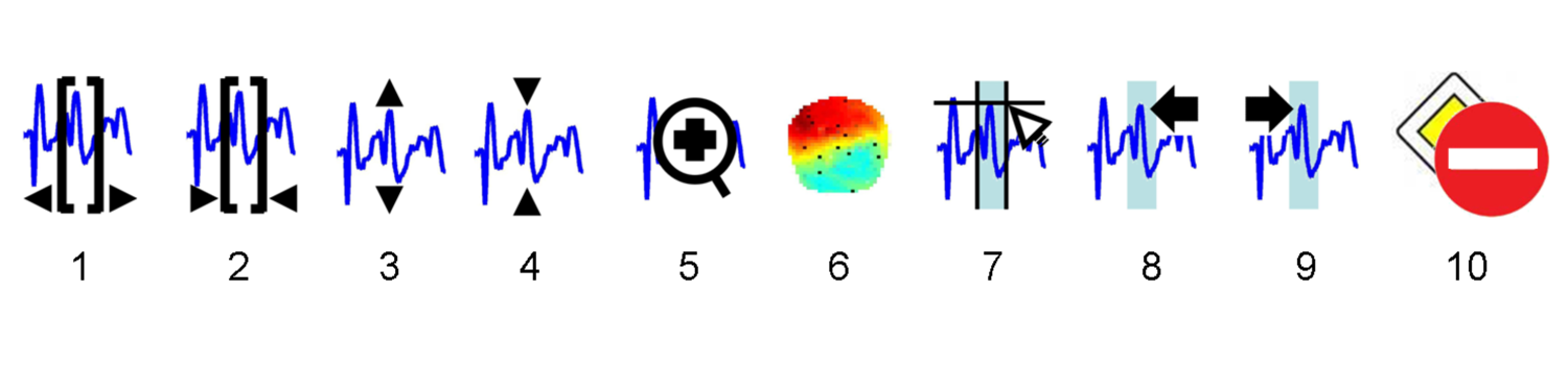
- standard channels are displayed vertically, within the same axes. A channel uicontextmenu can be accessed by right clicking on any time series (e.g. for changing the channel good/bad status). An additional axis (bottom right) provides the user with the temporal and horizontal scale of the displayed data). The size of the plotted time window can be changed using the top left buttons 1 and 2. User can scroll through the data using the temporal slider, at the bottom of the graphics window. A global display scaling factor can be changed using the top buttons 3 and 4. Zooming within the data is done by clicking on button 5. Clicking on button 6 displays a 2D scalp projection of the data.
When displaying epoched data, the user can select the trial within the list of accessible trials (top right of the window). It is also possible to switch the status of trials (good/bad) by clicking on button 10.
When displaying continuous data, SPM M/EEG Review allows the user to manage events and selections. After having clicked on button 7, the user is asked to add a new event in the data file, by specifying its temporal bounds (two mouse clicks within the display axes). Basic properties of any events can be accessed either in the “info” table, or by right-clicking on the event marker (vertical line or patch superimposed on the displayed data). This gives access to the event uicontextmenu (e.g. for changing the event label). Buttons 8 and 9 allow the user to scroll through the data from marker to marker (backward and forward in time).
- scalp channels are displayed vertically, within the same axes. A channel uicontextmenu can be accessed by right clicking on any time series (e.g. for changing the channel good/bad status). An additional axis (bottom right) provides the user with the temporal and horizontal scale of the displayed data). The size of the plotted time window can be changed using the top left buttons 1 and 2. User can scroll through the data using the temporal slider, at the bottom of the graphics window. A global display scaling factor can be changed using the top buttons 3 and 4. Zooming within the data is done by clicking on button 5. Clicking on button 6 displays a 2D scalp projection of the data.
When displaying epoched data, the user can select the trial within the list of accessible trials (top right of the window). It is also possible to switch the status of trials (good/bad) by clicking on button 10.
Source reconstructions visualization
SPM M/EEG Review makes use of sub tabs for any source reconstruction that has been stored in the data file7. Since these reconstructions are associated with epoched data, the user can choose the trial he/she wants to display using the list of accessible events (top of the main tab). Each sub tab has a label given by the corresponding source reconstruction comment which is specified by the user when source reconstructing the data (see relevant section in the SPM manual). The bottom-left part of each sub tab displays basic infos about the source reconstruction (date, number of included dipoles, number of temporal modes, etc). The top part of the window displays a rendering of the reconstruction on the cortical surface that has been used. User can scroll through peri-stimulus time by using the temporal slider below the rendered surface. Other sliders allow the user to (i) change the transparency of the surface (left slider) and (ii) threshold the colormap (right sliders). In the center, a butterfly plot of the reconstructed intensity of cortical source activity over peri-stimulus time is displayed. If the data file contains more than one source reconstruction, the bottom-right part of the window displays a bar graph of the model evidences of each source reconstruction. This provides the user with a visual Bayesian model comparison tool8. SPM M/EEG Review allows quick and easy switching between different models and trials, for a visual comparison of cortical source activities.
Script generation
Another way of batching jobs is by using scripts, written in MATLAB .
You can generate these scripts automatically. To do this, you first have
to analyze one data set using the GUI or batch system. Whenever a
preprocessing function is called, all the input arguments, once they
have been assembled by the GUI, are stored in a “history”. This history
can then be used to not only see in detail which functions have been
used on a data set, but also to generate a script that repeats the same
analysis steps. The big difference is that, this time, no more GUI
interactions are necessary because the script already has all the input
arguments which you gave during the first run. The history of an meeg
object can be accessed by D.history.
To generate a script from the history of an SPM MEEG file, open the file
in the M/EEG Review facility and select
the info tab: a history tab is then available that will display all
the history of the file. Clicking the Save as
script button will ask for the filename of the MATLAB script to
save and the list of processing steps to save (default is all but it is
possible to select only a subset of them). This will generate a script,
which, when run, repeats the analysis. The script can also be obtained
by directly calling the function spm_eeg_history.
Of course, this script can not only be used to repeat an analysis, but
the script can also be seen as a template that can be reused for other
analyses. One needs minimal MATLAB knowledge for these changes. For
example, you can replace the filenames to preprocess a different
subject. Or you can change parameters and then re-run the analysis. We
have prepared an example, using the same example data set, as in the
previous subsection to demonstrate this (see the file
man\(\backslash\)example_scripts\(\backslash\)history_subject1.m).
With a script, you could also use object methods directly, e.g. add a
line like D=badchannels(D, 23, 1), which flags channel 23 as bad (see
also our example script after the filtering step). To run the example
script on your computer, you need the data set that you can download
from the SPM webpage (9).
-
FieldTrip: http://fieldtrip.fcdonders.nl/ ↩
-
Users can also check sensor coregistration when clicking on “sensor positions”. ↩
-
Sensor/trial status (good/bad) can also be changed under the EEG/MEG/OTHER tabs, when visualizing trials (sensor: right-click uicontextmenu ; trials: button 10). ↩
-
This is part of the SPM EEG preprocessing tools. It mainly concerns the coregistration of the sensors onto the normalized SPM space. See relevant section in the SPM manual. ↩
-
This concerns any distributed source reconstruction, i.e. also includes imaging DCM analyses, but not ECD reconstructions (so far). ↩
-
Remember that model evidences \(p(y|m)\) can only be compared for the same data. Therefore, if the source reconstructions have different time windows, filters, number of temporal modes, etc., the comparison does not hold. This is why basic information (bottom-left part of the window) has to be recalled when comparing models. ↩