Statistical Analysis
For MSc Advanced Neuroimaging students
MSc Advanced Neuroimaging students should work with the images from the processed folder and use the pre-prepared info.txt file.
Others will need to preprocess a load of scans and generate their own info.txt file.
Now we are ready to fit a general linear model through the processed data (Friston et al, 1994), and make inferences (Worsley et al, 1996) about where there are systematic differences among the processed data.
The idea now is to set up a linear model in which to interpret any differences among the processed data. A different model will give different results, so in publications it is important to say exactly what was included. Similarly, the models used for processing also define how findings are interpreted. Grey matter is defined as what the segmentation model says it as. Homologous structures are defined by what the registration model considers homologous. The amount of smoothing also defines something about what the scale at which the data is examined. Changes to any of these components will generate slightly different processed data, and therefore a different pattern of results.
Returning to the analysis at hand, the strategy is:
-
Use Basic Models to specify a design matrix that explains how the processed data are caused.
-
Use Review models, to see what is in the design matrix, and generally poke about.
-
Use Estimate to actually fit the multiple regression to the data, and estimate the smoothness of the residuals for the subsequent random field theory corrections.
-
Use Results to characterise differences.
Basic Models
Click the Basic Models button on the top-left figure with the buttons on it (or select Stats and Factorial design specification via the batching system). This will give a whole list of options about Directory, Design, Covariates, Multiple covariates, Masking, Global calculation and Global normalisation.
Directory
The statistics part of SPM generally involves producing a bunch of results that are all saved in some particular directory. If you run more than one analysis in the same directory, then the results of the later analyses will overwrite the earlier results (although you do get a pop-up that asks whether or not you wish to continue). The Directory option is where you specify a directory in which to run the analysis (so create a suitable one first).
Global Calculation
For VBM, the “global normalisation” is about dealing with brains of different sizes. Because VBM is a voxel-wise assessment of volumetric differences, then it is useful to consider how the regional volumes are likely to vary as a function of whole brain volume. Bigger brains are likely to have larger brain structures. In a comparison of two populations of subjects, if one population has larger brains than the other, then should we be surprised if we find lots of volumetric differences? By including some form of correction for the “global” brain volume, then we may obtain more focused results.
So what measure should be used to do the correction?
Favourite measures are total grey matter volume, whole brain volume (with or without including the cerebellum) and total intra-cranial volume.
Within the aging and dementia research fields, total intra-cranial volume is the most accepted measure, but other researchers may favour different ones.
“Globals” can be computed in a number of ways.
For example, obtaining the total volume of grey matter could be achieved by adding up the values in a c1 or mwc1 image, and multiplying by the volume of each voxel.
Similarly, whole brain volume can be obtained by adding together the volume of grey matter and white matter.
Total intra-cranial volume can be obtained by adding up grey matter, white matter and CSF volumes.
The SPMUtilsTissue Volumes option from the batching system can be used to compute these.
A set of values that can be used as “globals” have been provided, which were obtained by summing up the volumes of grey matter, white matter and CSF.
These values can be loaded into MATLAB by loading the info.txt file, which is a simple text file.
If it is in your current directory, you can do this by typing the following into MATLAB:
This will load the contents of the file into a variable called info (same variable name as file name). In MATLAB, you can see the values of this variable by typing:
Among other things, this variable encodes the values that we’ll use as globals. Note that it contains 55 rows, which is the same as the number of scans to be entered into the statistical analysis. Click on Global calculation, and choose User, which indicates user-specified values. A User option should now have appeared, which has a field that says Global values. Select this, so a box should appear, in which you can enter the values of the globals. To do this, enter
This indicates that the sum of columns 3, 4 and 5 of the info variable should be used.
Global Normalisation
This part indicates how the “globals” should be used. Overall grand mean scaling should be set to No. Then click Normalisation, to reveal options about how our “globals” are to be used.
-
None indicates that no “global” correction should be done.
-
Proportional scaling indicates that the data should be divided by the “globals”. If the “globals” indicate whole brain volume, then this scales the values in the processed data so that they are proportional to the fraction of brain volume accounted for by that piece of grey matter. Similar principles apply when other values are used for “globals”.
-
ANCOVA correction simply treats the “globals” as covariates in the GLM. The results will show differences that can not be explained by the globals.
For this analysis, I suggest using proportional scaling.
Masking
Masking includes a number of options for determining which voxels are to be included in the analysis. The corrections for multiple comparisons mean that analyses are more sensitive if fewer voxels are included. For VBM studies, there are also instabilities that occur if the background is included in the analysis. In the background, there is little or no signal, so the estimated variance is close to zero. The t statistics are proportional to the magnitudes of the differences, divided by the square root of the residual variance. Division by zero, or numbers close to zero is problematic. Also, it is possible for blobs to extend out a long way into the background (see Ridgway et al, 2012), but this is prevented by the masking.
The parametric statistical tests within SPM assume that distributions are Gaussian. Another reason for masking is that values close to zero can not have Gaussian distributions, if they are constrained to be positive. If they were truly Gaussian, then at least some negative values should be possible.
It is possible to supply an image of ones and zeros, which acts as an Explicit Mask. The other masking strategies involve some form of intensity thresholding of the data. Implicit Masking involves assuming that a value of zero at some voxel, in any of the images, indicates an unknown value. Such voxels are excluded from the analysis.
The main way of masking VBM data is to use Threshold masking. At each voxel, if a value in any of the images falls below the threshold, then that voxel is excluded from the analysis. Note that with Proportional scaling correction, the values are divided by the globals prior to generating the mask.
For these data, I suggest using Absolute masking, with a threshold of 0.2.
Covariates
It is possible to include additional covariates in the model, but these will be specified elsewhere. I therefore suggest not adding any here.
Design
This the the part where the actual design matrix and data are specified. For the current data, the analysis can be specified as a Multiple Regression, so select this Design option. There are then three fields to specify: Scans, Covariates and Intercept.
Click Scans <-, and select the 55 previously computed smwc1 files (from the processed folder).
For Intercept, Specify Menu Item, Include Intercept. This will model a constant term in the design matrix.
Click Covariates, and then New “Covariate” two times.
The plan will be to model sex and age as covariates. Sex is usually treated as a categorical variable, but can be modelled as a covariate of ones and zeros.
Enter the covariates as follows.
1. Enter info(:,1) as the Vector, Age as the Name and No centering for Centering.
- Enter
info(:,2)as the Vector,Sexas the Name and No centering for Centering. Values of0indicate a female subject, and1indicates male.
All information should now be entered. You can save the job if you like (Save button).
Hit the Run button, and SPM will set up the necessary information to actually perform the statistical analysis.
This information is saved in a SPM.mat file.
Review
The Review button gives the chance to see what has been specified. If you notice any mistakes, then you can set up the analysis again. This is why it could be useful to save job files as you go.
Estimate
The Estimate button actually runs the analysis.
Click Estimate, select the SPM.mat file that has just been created, and then wait a while.
The first step is to fit the data at each voxel to some linear combination of the columns of the design matrix. This generates a series of beta images, where the first indicates the contribution of the first column, the second is the contribution of the second column etc.
There is also a ResMS image generated, which provides the necessary standard deviations for computing the t statistics.
The second step is to compute residual images, from which the smoothness of the data is computed. By default, these images are temporary, and are automatically deleted as soon as they are no longer needed.
That’s it. Pretty simple really.
Results
Once the GLM has been fitted, it is possible to use the information from the resulting beta and ResMS images (as well as the SPM.mat file) to generate images of t statistics.
Contrast vectors are specified, which indicate the linear combination of beta images to test.
These linear combinations are saved as con images, and the idea is to identify any regions that differ from zero in some statistical sense.
The t statistics themselves are saved in spmT images.
Because lots of voxels are examined, some correction for the number of tests is needed.
The processed data are spatially smooth, and voxels are correlated with their neighbours, so Gaussian random field theory is used to correct for multiple dependent comparisons (Worsley at al, 1996).
Click the Results button, and select the SPM.mat file.
This brings up the SPM contrast manager.
Click the t-contrasts button, and then Define new contrast.
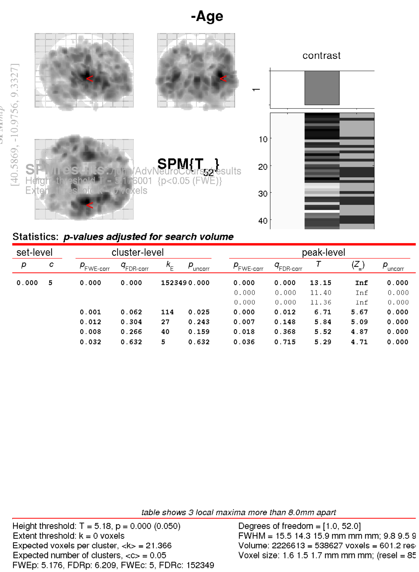
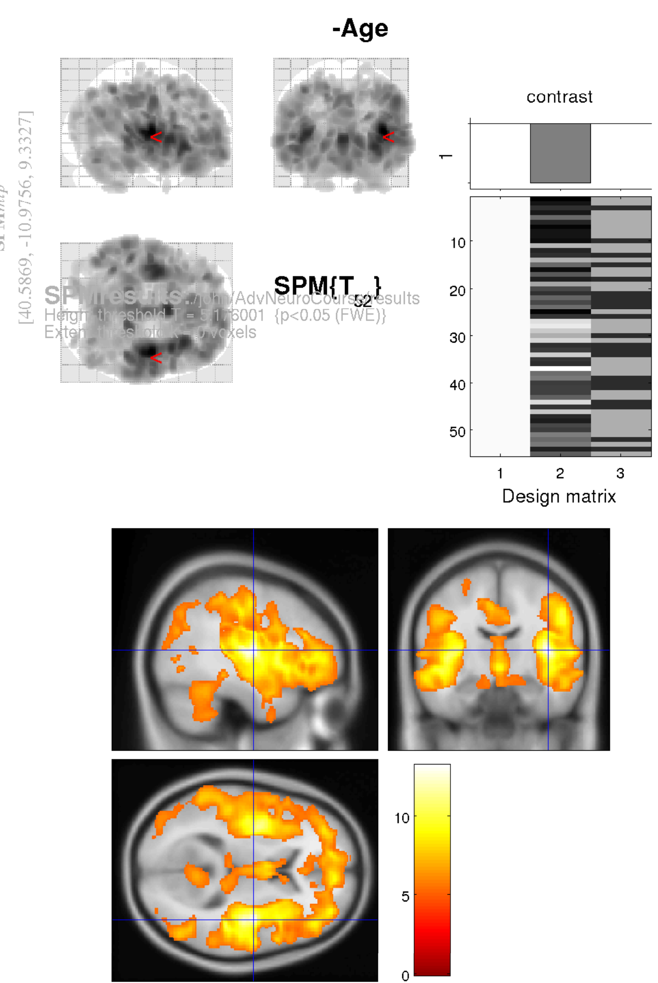
Enter -Age (or some other name of your choice) where the SPM contrast manager says name.
The idea is to test for regions with proportionally less grey matter in older subjects (i.e., more grey matter in younger subjects).
The t contrast for this is 0, -1, 0, 0. This would be entered into the field that says contrast.
Note that the trailing zero(s) can be omitted, as SPM will automatically fill these in.
Click OK, then click Done.
The lower-left SPM figure is now the one to focus on. This will prompt you for answers to a series of questions, so here goes.
-
mask with other contrast(s): click no.
-
title for comparison: leave this as it is. You can hit return on the keyboard, or click the edge of the text box with your mouse to do this.
-
p value adjustment to control: Click FWE (family-wise error correction).
-
threshold {T or p value}: Enter 0.05 for regions that are “statistically significant” after corrections for multiple comparisons (p<0.05).
-
& extent threshold {voxels}: lets see if there are any blobs at all, so go for
0.
Significance
Note that 0.05 is an arbitrary threshold to reach, with no mathematical or empirical justification, but it does seem to be one of those things that few seem to question (Nullius in verba as they say in the Royal Society). Some consider the 0.05 threshold to be much too lenient, and prefer 0.001. Some entire fields use thresholds of less than 10\(^{-6}\) (the 5\(\sigma\) criterion used by physicists – see http://www.dcscience.net/?p=6518). Laplace (who developed the Bayesian interpretation of probability) said “The weight of the evidence should be proportioned to the strangeness of the facts”, and some findings are certainly more surprising (“high-impact”) than others.
After waiting some time for the results to appear, you should see some blobs that show what is likely to happen to your brain in future.
To better understand the results, it is a good idea to examine the image files generated by the analysis. Check Reg can be used for this.