Multimodal face-evoked responses

Overview

This dataset contains EEG, MEG, functional MRI and structural MRI data on the same subject with the same paradigm, which allows a basic comparison of faces versus scrambled faces.

The dataset can be downloaded from the SPM website. It can be used to demonstrate, for example, 3D source reconstruction of various electrophysiological measures of face perception, such as the “N170” evoked response (ERP) recorded with EEG, or the analogous “M170” evoked field (ERF) recorded with MEG. These localisations are informed by the anatomy of the brain (from the structural MRI) and possibly by functional activation in the same paradigm (from the functional MRI).

The demonstration below involves localising the N170 using a distributed source method (called an “imaging” solution in SPM). The data can also be used to explore further effects, e.g. induced effects (Friston et al, 2006), effects at different latencies, or the effects of adding fMRI constraints on the localisation.

The EEG data were acquired on a 128 channel ActiveTwo system; the MEG data were acquired on a 275 channel CTF/VSM system; the sMRI data were acquired using a phased-array headcoil on a Siemens Sonata 1.5T; the fMRI data were acquired using a gradient-echo EPI sequence on the Sonata. The dataset also includes data from a Polhemus digitizer, which are used to coregister the EEG and the MEG data with the structural MRI.

Some related analyses of these data are reported in Henson et al (2005a, 2005b, 2007, 2009a, 2009b, in press), Kiebel and Friston (2004) and Friston et al (2006). To proceed with the data analysis, first download the data set from the SPM website[^1]. Most of the analysis below can be implemented in MATLAB 7.1 (R14SP3) and above. However, recoding condition labels using the GUI requires features of SPM8 only available in MATLAB 7.4 (R2007a) and above.

Paradigm and Data

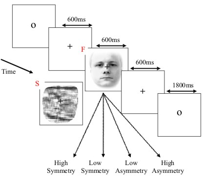
The basic paradigm involves randomised presentation of at least 86 faces and 86 scrambled faces Figure 1, based on Phase 1 of a previous study by Henson et al (2003). The scrambled faces were created by 2D Fourier transformation, random phase permutation, inverse transformation and outline-masking of each face. Thus faces and scrambled faces are closely matched for low-level visual properties such as spatial frequency content. Half the faces were famous, but this factor is collapsed in the current analyses. Each face required a four-way, left-right symmetry judgment (mean RTs over a second; judgments roughly orthogonal to conditions; reasons for this task are explained in Henson et al, 2003). The subject was instructed not to blink while the fixation cross was present on the screen.

One trial in the experiment. Trials involved either a Face (F) or Scrambled face (S).

Structural MRI

The T1-weighted structural MRI of a young male was acquired on a 1.5T Siemens Sonata via an MDEFT sequence with resolution \(1 \times 1 \times 1 mm^3\) voxels, using a whole-body coil for RF transmission and an 8-element phased array head coil for signal reception.

The images are in NIfTI format in the sMRI sub-directory, consisting of two files:

    sMRI/sMRI.img
    sMRI/sMRI.hdr

The structural was manually positioned to roughly match Talairach space, with the origin close to the Anterior Commissure. The approximate position of 3 fiducials within this MRI space - the nasion, and the left and right peri-aricular points - are stored in the file:

    sMRI/smri_fid.txt

These were identified manually (based on anatomy) and are used to define the MRI space relative to the EEG and MEG spaces, which need to be coregistered (see below). It doesn’t matter that the positions are approximate, because more precise coregistration is implemented via digitised surfaces of the scalp (“head shape functions”) that were created using the Polhemus 3D digitizer.

EEG data

The EEG data were acquired on a 128-channel ActiveTwo system, sampled at 2048 Hz, plus electrodes on left earlobe, right earlobe, and two bipolar channels to measure HEOG and VEOG. The 128 scalp channels are named: 32 A (Back), 32 B (Right), 32 C (Front) and 32 D (Left). The data acquired in two runs of the protocol are contained in two Biosemi raw data files:

    EEG/faces_run1.bdf
    EEG/faces_run2.bdf

The EEG directory also contains the following files:

    EEG/condition_labels.txt

This text file contains a list of condition labels in the same order as the trials appear in the two files - “faces” for presentation of faces and “scrambled” for presentation of scrambled faces. The EEG directory also contains the following files:

    EEG/electrode_locations_and_headshape.sfp

This ASCII file contains electrode locations, fiducials and headshape points measured with Polhemus digitizer.

The 3 fiducial markers were placed approximately on the nasion and preauricular points and digitised by the Polhemus digitizer. Later, we will coregister the fiducial points and the head shape to map the electrode positions in the “Polhemus space” to the “MRI space”. Also included as reference are some SPM batch files and SPM scripts (though these are recreated as part of the demo):

    EEG/batch_eeg_XYTstats.mat
    EEG/batch_eeg_artefact.mat
    EEG/eeg_preprocess.m
    EEG/faces_eeg_montage.m

MEG data

The MEG data were acquired on a 275 channel CTF/VSM system, using second-order axial gradiometers and synthetic third gradient for denoising and sampled at 480 Hz. There are actually 274 MEG channels in this dataset since the system it was recorded on had one faulty sensor. Two runs (sessions) of the protocol have been saved in two CTF datasets (each one is a directory with multiple files)

    MEG/SPM_CTF_MEG_example_faces1_3D.ds
    MEG/SPM_CTF_MEG_example_faces2_3D.ds

The MEG data also contains a headshape.mat file, containing the headshape recorded during the MEG experiment with a Polhemus digitizer.

The locations of the 3 fiducials in the headshape.mat file are the same as the positions of 3 “locator coils” the locations of which are measured by the CTF machine, and used to define the coordinates (in “CTF space”) for the location of the 274 sensors.

Also included as reference are two SPM batch files and two trial definition files (though these are recreated as part of the demo):

    MEG/batch_meg_preprocess.mat
    MEG/batch_meg_TFstats.mat
    MEG/trials_run1.mat
    MEG/trials_run2.mat

fMRI data

The fMRI data were acquired using a gradient-echo EPI sequence on a 3T Siemens TIM Trio, with 32, 3mm slices (skip 0.75mm) of \(3\times 3 mm^2\) pixels, acquired in a sequential descending order with a TR of 2s. There are 390 images in each of the two “Session” sub-directories (5 initial dummy scans have been removed), each consisting of a NIfTI image and header file:

    fMRI/Session1/fM*.{hdr,img}
    fMRI/Session2/fM*.{hdr,img}

Also provided are the onsets of faces and scrambled faces (in units of scans) in the MATLAB file:

    fMRI/trials_ses1.mat
    fMRI/trials_ses2.mat

and two example SPM batch files (see fMRI Section).

    fMRI/batch_fmri_preproc.mat
    fMRI/batch_fmri_stats.mat

Getting Started

You need to start SPM and toggle EEG as the modality (bottom-right of SPM main window), or start SPM with spm eeg. In order for this to work you need to ensure that the main SPM directory is on your MATLAB path.

EEG analysis

First change directory to the EEG subdirectory (either in MATLAB, or via Utils CD.

Convert

Select Convert Convert and select the faces_run1.bdf file. At the prompt Define settings? select just read. SPM will now read the original Biosemi format file and create an SPM compatible data file, called spmeeg_faces_run1.mat and spmeeg_faces_run1.dat in the current MATLAB directory. After the conversion is complete the data file will be automatically opened in SPM reviewing tool. By default you will see the info tab. At the top of the window there is some basic information about the file. Below it you will see several clickable tabs with additional information. The history tab lists the processing steps that have been applied to the file. At this stage there is only one such step - conversion. The channels tab lists the channels in the file and their properties, the trial tab lists the trials or in the case of a continuous file all the triggers (events) that have been recorded. The inv tab is used for reviewing the inverse solutions and is not relevant for the time being. At the top of the window there is another set of tabs. If you click on the EEG tab you will see the raw EEG traces. They all look unusually flat because the continuous data we have just converted contains very low frequencies and baseline shifts. Therefore, if we try to view all the channels together, this can only be done with very low gain. If you press the intensity rescaling button (with arrows pointing up and down) several times you will start seeing EEG activity in a few channels but the other channels will not be visible as they will go out of range. You can also use the controls at the bottom of the window to scroll through the recording. If you press the icon to the right of the mini-topography icon, with the rightwards pointing arrow, the display will move to the next trigger, shown as a vertical line through the display. (New triggers/events can be added by the rightmost icon). At the bottom of the display is a plot of the global field power across the session, with the black line indicating the current timewindow displayed (the width of this timewindow can be controlled by the two leftmost top icons).

Downsample

Here, we will downsample the data in time. This is useful when the data were acquired like ours with a high sampling rate of 2048 Hz. This is an unnecessarily high sampling rate for a simple evoked response analysis, and we will now decrease the sampling rate to 200 Hz, thereby reducing the file size by more than ten fold and greatly speeding up the subsequent processing steps. Select Preprocessing Downsample. In the batch window that will open, double click on File name and select the spmeeg_faces_run1.mat file. Then double click on New sampling rate and enter 200 for 200 Hz. The button will change its colour to green. Press it. The progress bar will appear and the resulting data will be saved to files dspmeeg_faces_run1.mat and dspmeeg_faces_run1.dat. Note that this dataset and other intermediate datasets created during preprocessing will not be automatically opened in the reviewing tool, but you can always review them by selecting Display M/EEG and choosing the corresponding .mat file.

Montage

In this step, we will identify the VEOG and HEOG channels, remove several channels that don’t carry EEG data and are of no importance to the following and convert the 128 EEG channels to “average reference” by subtracting the mean of all the channels from each channel¹. We generally recommend removal of data channels that are no longer needed because this will reduce the total file size and conversion to average reference is necessary for source modelling to work correctly. To do so, we use the Preprocessing Montage tool in SPM, which is a general approach for pre-multiplying the data matrix (channels \(\times\) time) by another matrix that linearly weights all channel data. This provides a very general method for data transformation in M/EEG analysis.

The appropriate montage-matrix can be specified in SPM by either using a graphical interface in the Convert Prepare tool, or by supplying the matrix saved in a file. We will do the latter. The script to generate this file is faces_eeg_montage.m. Running this script will produce a file named faces_eeg_montage.mat. In our case, we would like to keep only channels 1 to 128. To re-reference each of these to their average, the script uses MATLAB “detrend” to remove the mean of each column (of an identity matrix). In addition, there were four EOG channels (131, 132, 135, 136), where the HEOG is computed as the difference between channels 131 and 132, and the VEOG by the difference between channels 135 and 136.

You now call the montage function by choosing Preprocessing Montage and:

• Under File name' select the M/EEG-filedspm8_faces_run1.mat`.

• Make sure Write is selected for Mode and Load montage from file under Montage specification.

• Double click on Montage file name and select the generated faces_eeg_montage.mat file.

• Keep the other channels? should be set at No.

This will remove the uninteresting channels from the data. The progress bar appears and SPM will generate two new files Mdspmeeg_faces_run1.mat and Mdspmeeg_faces_run1.dat.

Epoch

To epoch the data select Preprocessing Epoch. Double click on File name and select the Mdspmeeg_faces_run1.mat file. For How to define trials select Define trial. And for Time window specify [-200 600]. Under Trial, click New. There is no information in the file at this stage to distinguish between faces and scrambled faces. We will add this information at a later stage. You can specify anything for Condition label, for instance “stim”. Event type and Event value might mean different things for different EEG and MEG systems. So you should be familiar with your particular system to find the right trigger for epoching. To explore a complete list of all events in the EEG file you can use the Convert Prepare tool selecting Batch inputs Event list. In our case, it is not very difficult as all the events but one appear only once in the recording, whereas the event with type “STATUS” and value 1 appears 172 times which is exactly the number of times a visual stimulus was presented. So in the batch window specify ‘STATUS’ for Event type and ‘1’ for Event value. Run the batch, The progress bar will appear and the epoched data will be saved to files eMdspmeeg_faces_run1.mat and eMdspmeeg_faces_run1.dat. The epoching function also performs baseline correction by default (with baseline -200 to 0ms). Therefore, in the epoched data the large channel-specific baseline shifts are removed and it is finally possible to see the EEG data clearly in the reviewing tool.

Reassignment of trial labels

Open the file eMdspmeeg_faces_run1.mat in the reviewing tool (under Display M\EEG ). The first thing you will see is that in the history tab there are now 4 processing steps. Now switch to the “trials” tab. You will see a table with 172 rows - exactly the number of events we selected before. In the first column the label “stim” appears in every row. What we would like to do now is change this label to “faces” or “scrambled” where appropriate. We should first open the file condition_labels.txt (in the EEG directory) with any text editor, such as MATLAB editor or Windows notepad. In this file there are exactly 172 rows with either “faces” or “scrambled” in each row. Unfortunately, with the latest changes in Matlab table interface, using GUI to update the labels is no longer possible and we’ll have to use the following code snipped to achieve the same effect:

D = spm_eeg_load('eMdspmeeg_faces_run1.mat')
D = conditions(D, ':', importdata('condition_labels.txt'));
save(D)

D is an object, this is a special kind of data structure that makes it possible to keep different kinds of related information (in our case all the properties of our dataset) and define generic ways of manipulating these properties. For instance we can use the command:

D = conditions(D, ':', importdata('condition_labels.txt'));

to update the trial labels using information imported from the condition_labels.txt². Now, conditions’ is a “method”, a special function that knows where to store the labels in the object. All the methods take the M/EEG object (usually called D in SPM by convention) as the first argument. The second argument is a list of indices of trials for which we want to change the label. We specify ‘:’ which is interpreted as “all”. The third argument is the new labels which are imported from the text file using a MATLAB built-in function. We then save the updated dataset on disk using the save method. If you now write D.conditions or conditions(D) (which are two equivalent ways of calling the conditions method with just D as an argument), you should see a list of 172 labels, either “faces” or “scrambled”.

If you reopen the file now in the reviewing tool, the new labels should now appear for all rows.

Using the history and object methods to preprocess the second file

At this stage we need to repeat the preprocessing steps for the second file faces_run2.bdf. You can do it by going back to the “Convert” section and repeating all the steps for this file, but there is a more efficient way. If you have been following the instructions until now the file eMdspmeeg_faces_run1.mat should be open in the reviewing tool. If it is not the case, open it. Go to the “history” tab and press the “Save as script” button. A dialog will appear asking for the name of the MATLAB script to save. Let’s call it eeg_preprocess.m. Then there will be another dialogue suggesting to select the steps to save in the script. Just press “OK” to save all the steps. Now open the script in the MATLAB editor. You will now need to make some changes to make it work for the second file. Here we suggest the simplest way to do it that does not require familiarity with MATLAB programming. But if you are more familiar with MATLAB you’ll definitely be able to do a much better job. First, replace all the occurrences of “run1” in the file with “run2”. You can use the “Find & Replace” functionality (Ctrl-F) to do it. Secondly, add the lines we previously used to update the trial labels at the end of the file (the two runs had identical trials).

D = conditions(D, ':', importdata('condition_labels.txt'));
save(D)

This is necessary because the steps done with custom code are not recorded in the file history. Save the changes and run the script by pressing the “Run” button or writing eeg_preprocess in the command line. SPM will now automatically perform all the steps we have done before using the GUI. This is a very easy way for you to start processing your data automatically once you come up with the right sequence of steps for one file. After the script finishes running there will be a new set of files in the current directory including eMdspmeeg_faces_run2.mat and eMdspmeeg_faces_run2.dat.

Merge

We will now merge the two epoched files we have generated until now and continue working on the merged file. Select Preprocessing Merge. Under File names select both eMdspmeeg_faces_run1.mat and eMdspmeeg_faces_run2.mat. There are additional options in the Merge tool to recode the condition labels but you can leave them at default meaning that the trial labels we have just specified will be copied as they are to the merged file. A new dataset will be generated called ceMdspmeeg_faces_run1.{mat,dat}.

Prepare

In this section we will add the separately measured electrode locations and headshape points to our merged dataset. In principle, this step is not essential for further analysis because SPM automatically assigns electrode locations for commonly used EEG caps and the Biosemi 128 cap is one of these. Thus, default electrode locations are present in the dataset already after conversion. But since these locations are based on channel labels they may not be precise enough and in some cases may be completely wrong because sometimes electrodes are not placed in the correct locations for the corresponding channel labels. This can be corrected by importing individually measured electrode locations. Select Convert Prepare and then File Open and in the file selection window select ceMdspmeeg_faces_run1.mat. A menu will appear at the top of SPM interactive window (bottom left window). Choose Sensors Load EEG sensors Convert locations file. In the file selection window choose the electrode_locations_and_headshape.sfp file (in the original EEG directory). Then from the “2D projection” submenu select “Project 3D (EEG)”. A 2D channel layout will appear in the Graphics window. Select 2D Projection Apply and File Save. Note that the same functionality can also be accessed from the reviewing tool by pressing the Prepare SPM file button.

Artefact rejection

Here we will use SPM artefact detection functionality to exclude from analysis trials contaminated with large artefacts. Select Preprocessing Detect artefacts. Click on File name and select the ceMdspmeeg_faces_run1.mat file. Double click How to look for artefacts and a new branch will appear. It is possible to define several sets of channels to scan and several different methods for artefact detection. We will use simple thresholding applied to all channels. Click on Detection algorithm and select Threshold channels in the small window below. Double click on Threshold and enter 200 (in this case \(\mu V\)). The batch is now fully configured. Run it by pressing the green button at the top of the batch window.

This will detect trials in which the signal recorded at any of the channels exceeds 200 microvolts (relative to pre-stimulus baseline). These trials will be marked as artefacts. Most of these artefacts occur on the VEOG channel, and reflect blinks during the critical time window. The procedure will also detect channels in which there is a large number of artefacts (which may reflect problems specific to those electrodes, allowing them to be removed from subsequent analyses).

In this case, the MATLAB window will show:

    There isn't a bad channel.
    39 rejected trials: 38   76   82   83   86   88   89   90   92   [...]

(leaving 305 valid trials). A new file will also be created, aceMdspm8_faces_run1.{mat,dat}.

Exploring the M/EEG object

We can now review the preprocessed dataset from the MATLAB command line by typing:

    D = spm_eeg_load

and selecting the aceMdspmeeg_faces_run1.mat file. This will print out some basic information about the M/EEG object D that has been loaded into MATLAB workspace.

    SPM M/EEG data object
    Type: single
    Transform: time
    2 conditions
    130 channels
    161 samples/trial
    344 trials
    Sampling frequency: 200 Hz
    Loaded from file  ...\EEG\aceMdspmeeg_faces_run1.mat
    Use the syntax D(channels, samples, trials) to access the data.

Note that the data values themselves are memory-mapped from aceMdspmeeg_faces_run1.dat and can be accessed by indexing the D object (e.g, D(1,2,3) returns the field strength in the first sensor at the second sample point during the third trial). You will see that there are 344 trials (D.ntrials). Typing D.conditions will show the list of condition labels consisting of 172 faces (“faces”) and 172 scrambled faces (“scrambled”). D.badtrials will return a \(1\times 39\) vector of indices of the rejected trials. D.condlist will display a list of unique condition labels. The order of this list is important because every time SPM needs to process the conditions in some order, this will be the order. If you type D.chanlabels, you will see the order and the names of the channels. D.chantype will display the type for each channel (in this case either “EEG” or “EOG”). D.size will show the size of the data matrix, [130 161 344] (for channels, samples and trials respectively). The size of each dimension separately can be accessed by D.nchannels, D.nsamples and D.ntrials. Note that although the syntax of these commands is similar to those used for accessing the fields of a struct data type in MATLAB, what’s actually happening here is that these commands evoke special functions called “methods” and these methods collect and return the requested information from the internal data structure of the D object. The internal structure is not accessible directly when working with the object. This mechanism greatly enhances the robustness of SPM code. For instance you don’t need to check whether some field is present in the internal structure. The methods will always do it automatically or return some default result if the information is missing without causing an error.

Type methods(’meeg’) for the full list of methods performing operations with the object. Type help meeg/method_name to get help about a method.

Basic ERPs

Select Average Average and select the aceMdspmeeg_faces_run1.mat file under File name. At this point you can perform either ordinary averaging or “robust averaging” (Wager et al., 2005). Robust averaging makes it possible to suppress artefacts automatically without rejecting trials or channels completely, but just the contaminated parts. Thus, in principle, we could do robust averaging without rejecting trials with eye blinks and this is something you can do as an exercise and see how much difference the artefact rejection makes with ordinary averaging vs. robust averaging. For robust averaging select Robust under Averaging type ³.

Finally,run the batch. A new dataset will be generated maceMdspmeeg_faces_run1.{mat,dat} (“m” for “mean”) and automatically opened in the reviewing tool so that you can examine the ERP.

Select Average Contrast. This function creates linear contrasts of ERPs/ERFs. Select the maceMdspmeeg_faces_run1.mat file, and create two new contrats, one with coefficients \([1\: -1]\) and label “Difference”,and another with coefficients \([1/2\: 1/2]\) and label “Mean”. Set Weight by replications to No and run the batch. This will create new file wmaceMdspmeeg_faces_run1.{mat,dat}, in which the first trial-type is now the differential ERP between faces and scrambled faces, and the second trial-type is the average ERP for faces and scrambled faces.

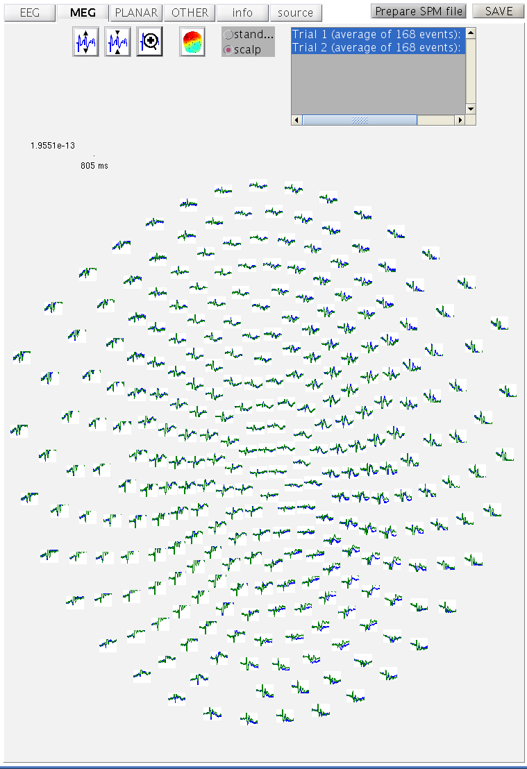
To look at the differential ERP, again select Display M/EEG, and select the wmaceMdspmeeg_faces_run1.mat file. Switch to the EEG tab and to scalp display by toggling a radio button at the top of the tab. The Graphics window should then show the ERP for each channel (for Trial 1 the “Difference” condition). Hold SHIFT and select Trial 2 to see both conditions superimposed. Then click on the zoom button and then on one of the channels (e.g, “B9” on the bottom right of the display) to get a new window with the data for that channel expanded, as in Figure 2.

Average (green) and differential (blue) ERPs for faces and scrambled faces at channel B9 in `wmaceMdspmeeg_faces_run1.mat`

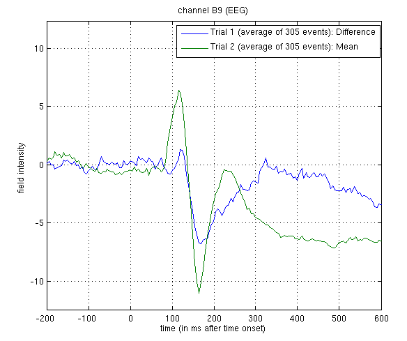
The green line shows the average ERP evoked by faces and scrambled faces (at this occipitotemporal channel). A P1 and N1 are clearly seen. The blue line shows the differential ERP between faces and scrambled faces. The difference is small around the P1 latency, but large and negative around the N1 latency. The latter likely corresponds to the “N170” (Henson et al, 2003). We will try to localise the cortical sources of the P1 and N170 in the section on 3D source reconstruction.

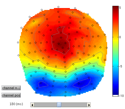
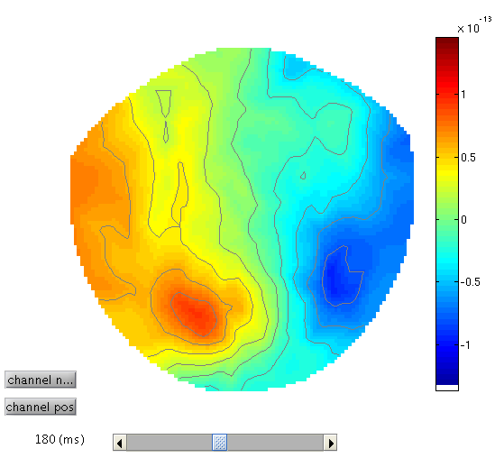
To see the topography of the differential ERP, click on Trial 1 again, press the “topography” icon button at the top of the window and scroll the latency from baseline to the end of the epoch. You should see a maximal difference around 180ms as in Figure 3 (possibly including a small delay of about 8ms for the CRT display to scan to the centre of the screen).

2D topography for faces minus scrambled faces at 180ms.

3D SPMs (Sensor Maps over Time)

A feature of SPM is the ability to use Random Field Theory to correct for multiple statistical comparisons across N-dimensional spaces. For example, a 2D space representing the scalp data can be constructed by flattening the sensor locations (using the 2D layout we created earlier) and interpolating between them to create an image of \(M\times M\) pixels (when \(M\) is user-specified, eg \(M=32\)). This would allow one to identify locations where, for example, the ERP amplitude in two conditions at a given timepoint differed reliably across subjects, having corrected for the multiple t-tests performed across pixels. That correction uses Random Field Theory, which takes into account the spatial correlation across pixels (i.e, that the tests are not independent). This kind of analysis is described earlier in the SPM manual, where a 1st-level design is used to create the images for a given weighting across timepoints of an ERP/ERF, and a 2nd-level design can then be used to test these images across subjects.

Here, we will consider a 3D example, where the third dimension is time, and test across trials within the single subject. We first create a 3D image for each trial of the two types, with dimensions \(M\times M\times S\), where S=161 is the number of samples. We then take these images into an unpaired t-test across trials (in a 2nd-level model) to compare faces versus scrambled faces. We can then use classical SPM to identify locations in space and time in which a reliable difference occurs, correcting across the multiple comparisons entailed. This would be appropriate if, for example, we had no a priori knowledge where or when the difference between faces and scrambled faces would emerge⁴.

Select Images Convert to images, and select the aceMdspmeeg_faces_run1.mat file. Under Mode select scalp x time. Under Channel selection choose Select channels by type EEG. Then click again on Channel selection and scroll to the bottom of the menu below to ‘Delete: All(1)’ item and click on it. This is the way in batch to remove the default option of using all the channels. Then you can run the batch.

It will take some time as it writes out an image for each trial (except rejected trials), in a new directory called aceMdspmeeg_faces_run1, which will contain two files

condition_faces.nii
condition_scrambled.nii

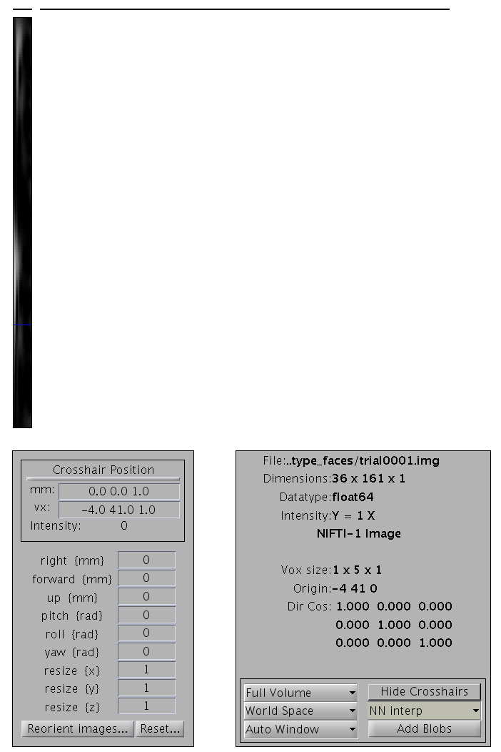
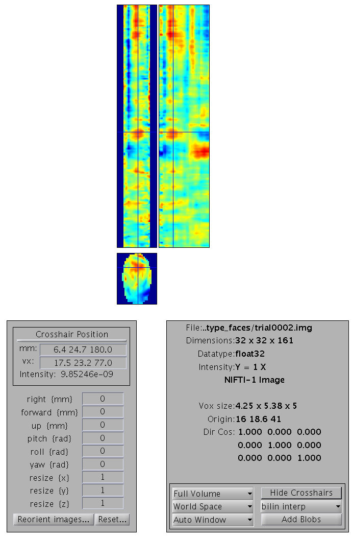
one for each trialtype. These are 4D NIfTI files with the dimensions being X and Y on the scalp, time and trials. You can press Display Image to view one of these images. By default, only the first trial/frame is shown. You can change that by modifying the value in the Frames box. If you set the value to inf as shown in Figure 3, all the frames will appear as a list that you can choose from. It might be helpful to combine this option with the use of the Filter box that allows to select frames from only one condition to be displayed by the use of regular expressions (e.g. faces to only see the frames for faces).

Interface for selecting trials/frames from 4D NIfTI

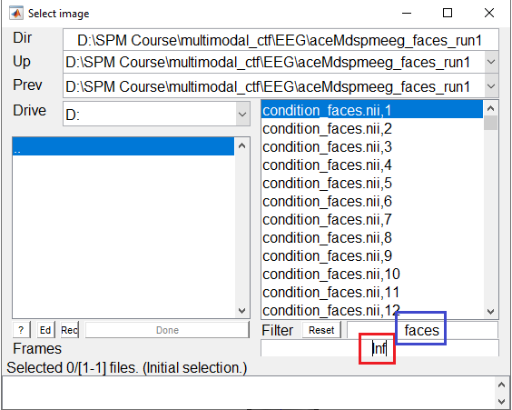
You can select any of the frames and examine it in the image viewer. It will have dimensions \(32\times 32\times 161\), with the origin set at [16 18.6 41] (where 41 samples is 0ms), as in Figure 4

3D image for a single trial of `aceMdspm8_faces_run1.mat`. The bottom image is a 2D x-y space interpolated from the flattened electrode locations (at one point in time). The two top images are sections through x and y respectively, now expressed over time (vertical (z) dimension).

Smoothing

Note that you can also smooth these images in 3D (i.e, in space and time) by selecting Images Smooth images. When you get the Batch Editor window, you can enter a smoothness of your choice (eg [9 9 20], or 9mm by 9mm by 20ms). Note that you should also change the default “Implicit masking” from “No” to “Yes”; this is to ensure that the smoothing does not extend beyond the edges of the topography.

As with fMRI, smoothing can improve statistics if the underlying signal has a smoothness close to the smoothing kernel (and the noise does not; the matched filter theorem). Smoothing may also be necessary if the final estimated smoothness of the SPMs (below) is not at least three times the voxel size; an assumption of Random Field Theory. In the present case, the data are already smooth enough (as you can check below), so we do not have to smooth further.

Stats

To perform statistics on these images, first create a new directory, eg. mkdir XYTstats.

Then press the “Specify 2nd level” button, to produce the batch editor window again. Select the new XYTstats as the “Directory”, and “two-sample t-test” (unpaired t-test) as the “Design”. Then select the frames from “condition_faces.nii” for ‘Group 1 scans’. To do that, you should make all the frames visible by entering inf in the Frames box and faces in the Filter box. It might be a good idea to first enter the filter string so that you can make sure that only the file you wanted to select is visible and only then expand it to frame list. Then right-click on the frames list and press Select All in the pop-up menu. Follow similar steps to select all the frames from “condition_scrambled.nii” for Group 2 scans. You might want to save this batch specification, but then press ⁵.

This will produce the design matrix for a two-sample t-test.

Then press Estimate, choose the “SPM.mat” from XYTstats file and run the batch. When it has finished, press “Results”, select the same “SPM.mat” and define a new F-contrast as [1 -1]. Keep the default contrast options, but threshold at \(p<.05\) FWE corrected for the whole search volume and select “Scalp-Time” for the “Data Type”. Then press “whole brain”, and the Graphics window should now look like that in Figure 5.

3D sensor-time SPM F at p<.05 FWE corrected for the amplitude difference between face and scrambled face trials. The x, y coordinates refer to position in the 32x32 electrode plane (with units of mm); the z coordinate refers to peristimulus time in ms (to the nearest sampling of 5ms).

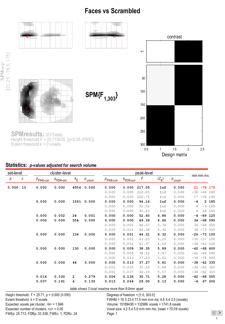
This will reveal “regions” within the 2D sensor space and within the -200ms to 600ms epoch in which faces and scrambled faces differ reliably, having corrected for multiple F-tests across pixels and time. There are a number of such regions, but the largest has maxima at [-13 -78 180] and [21 -68 180], corresponding to left and right posterior sites at 180ms.

To relate these coordinates back to the original sensors, right-click in some white space in the top half of the Graphics window, to get a menu with various options. First select “goto global maxima”. The red cursor should move to coordinates [21, -78, 175]. Then right-click again to get the same menu, but this time select “go to nearest suprathreshold channel”. You will be asked to select the original EEG/MEG file used to create the SPM, which in this case is the aceMdspmeeg_faces_run1.mat file. This should output in the Matlab window:

spm_mip_ui: Jumped 4.25mm from [ 21, -78, 175], to nearest suprathreshold channel (A28) at [ 17, -78, 175]

In other words, it is EEG channel “A28” that shows the greatest face/scrambled difference over the epoch (itself maximal at 175ms).

Note that you can also overlap the sensor names on the MIP by selecting display/hide channels. If the display gets too crowded you can zoom in.

Note that an F-test was used because the sign of the difference reflects the polarity of the ERP difference, which is not of primary interest (and depends on the choice of reference). Indeed, if you plot the contrast of interest from the cluster maxima, you will see that the difference is negative for the first posterior, cluster but positive for the second, central cluster. This is consistent with the polarity of the differences in Figure 3⁶.

If one had more constrained a priori knowledge about where and when the N170 would appear, one could perform an SVC based on, for example, a box around posterior channels and between 150 and 200ms poststimulus. See 3D Sensor SPMs page for more details.

If you go to the global maximum, then press overlays, sections and select the mask.img in the stats directory, you will get sections through the space-time image. A right click will reveal the current scalp location and time point. By moving the cursor around, you can see that the N170/VPP effects start to be significant (after whole-image correction) around 150ms (and may also notice a smaller but earlier effect around 100ms).

3D “imaging” reconstruction

Here we will demonstrate a distributed source reconstruction of the N170 differential evoked response between faces and scrambled faces, using a grey-matter mesh extracted from the subject’s MRI, and the Multiple Sparse Priors (MSP) method in which multiple constraints on the solution can be imposed (Friston et al, 2008, Henson et al, 2009a).

Press the 3D source reconstruction button, and press the load button at the top of the new window. Select the wmaceMdspmeeg_faces_run1.mat file and type a label (eg "N170 MSP") for this analysis⁷.

Press the “MRI” button, select the smri.img file within the sMRI sub-directory, and select normal for the cortical mesh.

The “imaging” option corresponds to a distributed source localisation, where current sources are estimated at a large number of fixed points (8196 for a “normal” mesh here) within a cortical mesh, rather than approximated by a small number of equivalent dipoles (the ECD option). The imaging approach is better suited for group analyses and (probably) for later-occuring ERP components. The ECD approach may be better suited for very early sensory components (when only small parts of the brain are active), or for DCMs using a small number of regions (Kiebel et al, 2006).

The first time you use a particular structural image for 3D source reconstruction, it will take some time while the MRI is segmented (and normalisation parameters determined). This will create in the sMRI directory the files y_smri.nii and smri_seg8.mat for normalisation parameters and 4 GIfTI (.gii) files defining the cortical mesh, inner skull, outer skull and scalp surface.

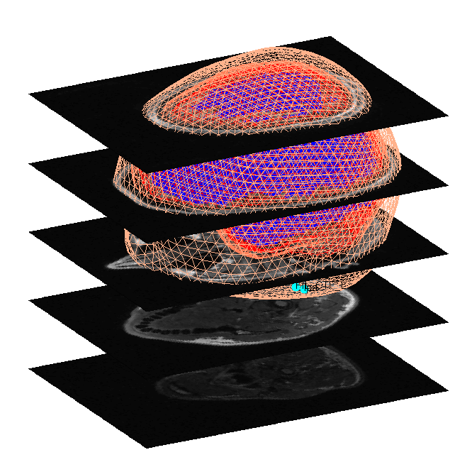
When meshing has finished, the cortex (blue), inner skull (red), outer skull (orange) and scalp (pink) meshes will be shown in the Graphics window with slices from the sMRI image, as shown in Figure 6. This makes it possible to visually verify that the meshes fit the original image well. The field D.inv{1}.mesh field will be updated in MATLAB . Press save in top right of window to update the corresponding mat file on disk.

Cortex (blue), inner skull (red), outer skull (orange) and scalp (pink) meshes with transverse slices of the subject’s MRI.

Both the cortical mesh and the skull and scalp meshes are not created directly from the segmented MRI, but rather are determined from template meshes in MNI space via inverse spatial normalisation (Mattout et al, 2007).

Press the Co-register button. You will first be asked to select at least 3 fiducials from a list of points in the EEG dataset (from Polhemus file): by default, SPM has already highlighted what it thinks are the fiducials, i.e, points labelled “nas” (nasion), “lpa” (left preauricular) and “rpa” (right preauricular). So just press “ok”.

You will then be asked for each of the 3 fiducial points to specify its location on the MRI images. This can be done by selecting a corresponding point from a hard-coded list (“select”). These points are inverse transformed for each individual image using the same deformation field that is used to create the meshes. The other two options are typing the MNI coordinates for each point (“type”) or clicking on the corresponding point in the image (“click”). Here, we will type coordinates based on where the experimenter defined the fiducials on the smri.img. These coordinates can be found in the smri_fid.txt file also provided. So press “type” and for “nas”, enter [0 91 -28]; for “lpa” press “type” and enter [-72 4 -59]; for “rpa” press “type” and enter [71 -6 -62]. Finally, answer “no” to “Use headshape points?” (in theory, these headshape points could offer better coregistration, but in this dataset, the digitised headshape points do not match the warped scalp surface very well, as noted below, so just the fiducials are used here).

This stage coregisters the EEG sensor positions with the structural MRI and cortical mesh, via an approximate matching of the fiducials in the two spaces, followed by a more accurate surface-matching routine that fits the head-shape function (measured by Polhemus) to the scalp that was created in the previous meshing stage via segmentation of the MRI. When coregistration has finished, a figure like that in Figure 7 will appear in the top of the Graphics window, which you can rotate with the mouse (using the Rotate3D MATLAB Menu option) to check all sensors. Finally, press save in top right of window to update the corresponding mat file on disk.

Graphical output of Co-registration of EEG data, showing (upper panel) cortex (blue), inner skull (red) and scalp (black) meshes, electrode locations (green), MRI/Polhemus fiducials (cyan/magneta), and headshape (red dots).

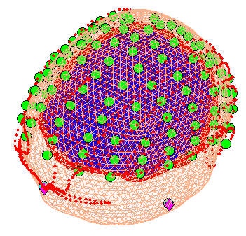
Note that for these data, the coregistration is not optimal, with several EEG electrodes appearing inside the scalp. This may be inaccurate Polhemus recording of the headshape or inaccurate surface matching for the scalp mesh, or “slippage” of headpoints across the top of the scalp (which might be reduced in future by digitising features like the nose and ears, and including them in the scalp mesh). This is not actually a problem for the BEM calculated below, however, because the electrodes are re-projected to the scalp surface (as a precaution).

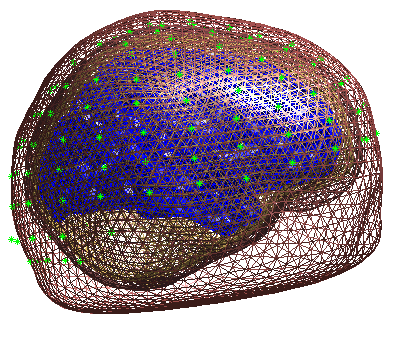
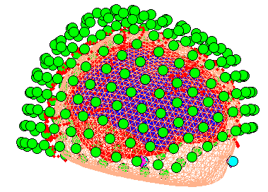
Press Forward Model, and select EEG BEM. The first time you do this, there will be a lengthy computation and a large file smri_EEG_BEM.mat will be saved in the sMRI directory containing the parameters of the boundary element model (BEM). In the Graphics window the BEM meshes will be displayed with the EEG sensors marked with green asterisks as shown (after rotating to a “Y-Z” view using MATLAB rotate tool) in Figure 8. This display is the final quality control before the model is used for lead field computation.

BEM meshes with the EEG sensors marked as asterisks.

Press Invert, select Imaging (i.e, a distributed solution rather than DCM; Kiebel et al (2006)), select yes to include all conditions (i.e, both the differential and common effects of faces and scrambled faces) and then Standard to use the default settings.

By default the MSP method will be used. MSP stands for “Multiple Sparse Priors” (Friston et al. 2008a), and has been shown to be superior to standard minimum norm (the alternative IID option) or a maximal smoothness solution (like LORETA; the COH option) - see Henson et al (2009a). Note that by default, MSP uses a “Greedy Search” (GS) (Friston et al, 2008b), though the standard ReML (as used in Henson et al, 2007) can also be selected via the batch tool (this uses Automatic Relevance Determination - ARD).

The Standard option uses default values for the MSP approach (to customise some of these parameters, press Custom instead).

At the first stage of the inversion lead fields will be computed for all the mesh vertices and saved in the file SPMgainmatrix_wmaceMdspmeeg_faces_run1_1.mat. Then the actual MSP algorithm will run and the summary of the solution will be displayed in the Graphics window.

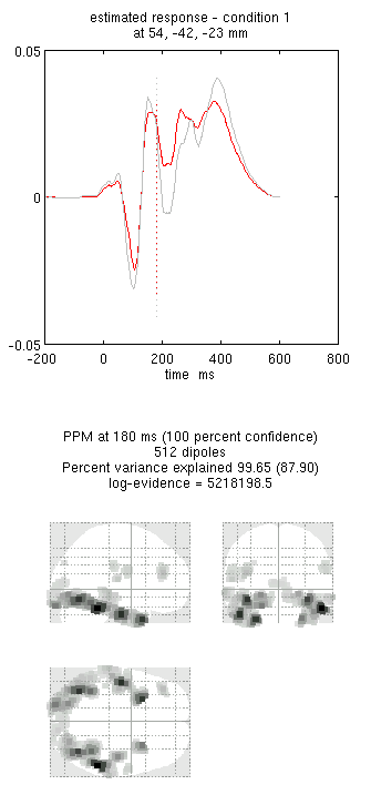
Press save to save the results. You can now explore the results via the 3D reconstruction window. If you type 180 into the box in the bottom right (corresponding to the time in ms) and press mip, you should see an output similar to Figure 9. This fit explains approx 96% of the data.

Graphical output of an MSP estimation of the differential ERP between faces and scrambled faces at 180ms

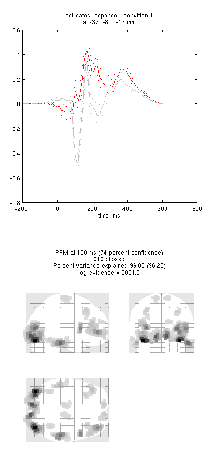
!!! tip “” Including several conditions in an inversion forces the algorithm to fit them all with the same set of sources. This is critical in this example because the “Difference” condition is likely to be too weak and noisy by itself to be reconstructed well. Combining it with the “Mean” that is generated by the same set of sources helps obtain a stable solution.

Note the hot-spots in bilateral posterior occipitotemporal cortex, bilateral mid-fusiform, and right lateral ventral temporal. The timecourses come from the peak voxel. The red curve shows the condition currently being shown (corresponding to the Condition 1 toggle bar in the reconstruction window); the grey line(s) will show all other conditions. Condition 1 is the differential evoked responses for faces vs scrambled; if you press the condition 1 toggle, it will change to Condition 2 (average evoked response for faces and scrambled faces), type “100”ms for the P100, then press mip again and the display will update (note the colours of the lines have now reversed from before, with red now corresponding to average ERP).

If you toggle back to Condition 1 and press movie, you will see changes in the source strengths for the differential response over peristimulus time (from the limits 0 to 300ms currently chosen by default). If you press render you can get a very neat graphical interface to explore the data (the buttons are fairly self-explanatory).

You can also explore other inversion options, such as COH and IID (available for the “custom” inversion), which you will notice give more superficial solutions (a known problem with standard minimum norm approaches). To do this quickly (without repeating the MRI segmentation, coregistration and forward modelling), press the new button in the reconstruction window, which by default will copy these parts from the previous reconstruction.

In this final section we will concentrate on how to prepare source data for subsequent statistical analysis (eg with data from a group of subjects).

Press the Window button in the reconstruction window, enter “150 200” as the timewindow of interest and keep “0” as the frequency band of interest (0 means all frequencies). The Graphics window will then show the mean activity for this time/frequency contrast (top plot) and the contrast itself (bottom plot; note additional use of a Hanning window).

Then press Image, select image as the output format and SPM will write 3D NIfTI images corresponding to the above contrast for each condition:

        wmaceMdspmeeg_faces_run1_1_t150_200_f_1.nii
        wmaceMdspmeeg_faces_run1_1_t150_200_f_2.nii

The last number in the file name refers to the condition number; the number following the dataset name refers to the reconstruction number (i.e. the number in red in the reconstruction window, i.e, D.val, here 1). The reconstruction number will increase if you create a new inversion by pressing new.

The smoothed results for Condition 1 (i.e, the differential evoked response for faces vs scrambled faces) will also be displayed in the Graphics window, see Figure 10 (after moving the cursor to the right posterior hotspot), together with the normalised structural. Note that the solution image is in MNI (normalised) space, because the use of a canonical mesh provides us with a mapping between the cortex mesh in native space and the corresponding MNI space.

3D reconstruction saved as a smoothed NIfTI image of the differential evoked response for faces vs scrambled faces around the N170.

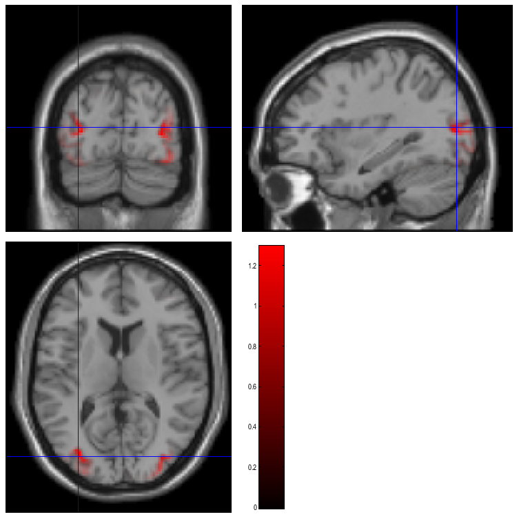
You can also of course view the image with the normal SPM Display Image option (just the functional image with no structural will be shown), and locate the coordinates of the “hotspots” in MNI space. Note that these images contain RMS (unsigned) source estimates (see Henson et al, 2007). Given that one has data from multiple subjects, one can create a NIFTI file for each. Group statistical analysis can the be implemented with eg. second level t-tests as described earlier in the chapter.

Since the images generated by inverting the “Difference” condition are nonnegative, it would not be statistically valid to enter them into a one-sample T-test. To do a statistical test at the second level images should be generated separately for “faces” and “scrambled” i.e. the maceMdspmeeg_faces_run1.mat should be inverted and then the pairs of images should be entered into a paired T-test design.

MEG analysis

Preprocessing the MEG data

First change directory to the MEG subdirectory (either in MATLAB, or via Utils CD)

Adjust trigger latency

For the EEG data, the faces were displayed directly via a CRT monitor. For the MEG data on the other hand, the faces were displayed inside the MSR via a projector. This projector produces a delay of 1.5 screen refreshes, which at 60Hz, is 25ms. This means that the subject actually saw the stimuli 25ms after the trigger was sent to the MEG acquisition machine. We can correct for the visual delay when doing the trial definition⁸. In the EEG case, we defined the trials at the epoching stage. Another way to do it is to define trials before conversion and read just the necessary segments from the data. This is especially useful when the epochs or interest comprise just a small fraction of the recording (e.g. in sleep studies). There is a slight problem, however, in that trial definition requires information about trigger timings from the dataset that has not been converted yet. To get around that, we will first convert just the dataset header containing all the meta-data related to the recording and then convert the dataset itself.

Select Convert Convert, navigate into SPM_CTF_MEG_example_faces1_3D.ds folder and select the SPM_CTF_MEG_example_faces1_3D.meg4 file. Answer yes to ‘define settings’. In the batch window that will open click on Reading mode and choose Header only from the menu. Run the batch. This will generate the file spmeeg_SPM_CTF_MEG_example_faces1_3D.mat.

Now select Convert Prepare. A menu will appear at the top of the interactive window (the small window at the bottom left). In that menu select File Open and choose the header file generated at the previous step. Then select Batch inputs Trial definition.

• Enter -200 600 for TIme window \[ms\]

• Enter 2 for How many conditions?.

• Enter “faces” for Label of condition 1. A dialog with a list of events will come up and Select the event with type UPPT001_up and Value 1.

• For Shift triggers (ms) enter 25 to shift by 25 ms as discussed above.

• Enter “scrambled” for Label of condition 2. Select the event with type UPPT001_up and Value 2.

• For Shift triggers (ms) enter 25 again.

• Answer no to the question about reviewing trials.

• Answer yes to the prompt to save the trial definition.

• Enter a filename like trials_run1.mat and save in the MEG directory.

Then type load trials_run1.mat in MATLAB, to see the contents of the file you just saved. It a few variables, including trl and conditionlabels. The trl variable contains as many rows as triggers were found (across all conditions) and three columns: the initial sample of the epoch, the final sample of the epoch and the offset in samples corresponding to a peristimulus time of 0. The sampling rate for the MEG data was 480Hz. Thus the figure of -96 samples in the third column corresponds to the 200ms baseline period that you specified.

Convert

Select Convert Convert, and in the file selection window again select theSPM_CTF_MEG_example_faces1_3D.dssubdirectory and theSPM_CTF_MEG_example_faces1_3D.meg4file. At the promptDefine settings?selectyes. Here we will use the option to define more precisely the part of data that should be read during conversion. ForReading mode, switch toEpoched. Click onEpochedand chooseTrial filein the menu. Then double click onTrial fileand in the file selector window, select the newtrials_run1.matfile. Run the batch. After the conversion is complete. You can open the datasetspmeeg_SPM_CTF_MEG_example_faces1_3D.matin the reviewing tool. If you click on theMEGtab you will see the MEG data which is already epoched. By pressing theintensity rescaling` button (with arrows pointing up and down) several times you will start seeing MEG activity.

Baseline correction

We need to perform baseline correction as it is not done automatically during conversion. This will prevent excessive edge artefacts from appearing after subsequent filtering and downsampling. Select Preprocessing Baseline-correct select the spmeeg_SPM_CTF_MEG_example_faces1_3D.mat file. Enter \([-200\: 0]\) for Baseline. The progress bar will appear and the resulting data will be saved to dataset bspmeeg_SPM_CTF_MEG_example_faces1_3D.{mat,dat}.

Downsample

Select Preprocessing Downsample. In the batch window that will open, double click on File name and select the spmeeg_SPM_CTF_MEG_example_faces1_3D.mat file. Then double click on New sampling rate and enter 200 for 200 Hz. Run the batch. The progress bar will appear and the resulting data will be saved to files dbspmeeg_SPM_CTF_MEG_example_faces1_3D.{mat,dat}.

Batch preprocessing

Here we will preprocess the second half of the MEG data using using the SPM batch facility. But first you should repeat the steps describe above to generate trial definition for the second recording block. You can save it in trials_run2.mat

Press the Batch button (lower right corner of the SPM menu window). The batch tool window will appear. We will define exactly the same settings as we have just done using the interactive GUI. From the “SPM” menu, “M/EEG” submenu select “M/EEG Conversion”. Click on File name and select the SPM_CTF_MEG_example_faces2_3D.meg4 file from SPM_CTF_MEG_example_faces2_3D.ds subdirectory. Click on Reading mode and switch to Epoched. Click on Epoched and choose Trial file, double-click on the new Trial file branch and then select the trials_run2.mat file. Then click on Channel selection and select MEG as done previously. Do not forget to delete the All setting.

Now select ‘Baseline correction’ from SPM M/EEG Preprocessing submenu. Another line will appear in the Module list on the left. Click on it. The baseline correction configuration branch will appear. Select File name with a single click. The file that we need to downsample has not been generated yet but we can use the Dependency button. A dialog will appear with a list of previous steps (in this case just the conversion) and we can set the output of one of these steps as the input to the present step. Now just enter enter \(-200\: 0\) for Baseline. Similarly we can now add Downsampling to the module list, define the output of baseline correction step for File name and 200 for the New sampling rate. This completes our batch. We can now save it for future use (e.g, as batch_meg_preprocess and run it by pressing the green button. This will generate all the intermediate datasets and finally dbspmeeg_SPM_CTF_MEG_example_faces2_3D.{mat,dat}.

Merge

We will now merge the two epoched files we have generated until now and continue working on the merged file. Select Preprocessing Merge. The merging is done similarly to what is described above for EEG. A new dataset will be generated called cdbspmeeg_SPM_CTF_MEG_example_faces1_3D.{mat,dat}.

Reading and preprocessing data using Fieldtrip

Yet another even more flexible way to pre-process data in SPM is to use the Fieldtrip toolbox that is distributed with SPM. All the pre-processing steps we have done until now can also be done in Fieldtrip and the result can then be converted to SPM dataset. An example script for doing so can be found in the man\(\backslash\)example_scripts\(\backslash\)spm_ft_multimodal_preprocessing.m. The script will generate a merged dataset and save it under the name ft_SPM_CTF_MEG_example_faces1_3D.{mat,dat}. The rest of the analysis can then be done as below. This option is more suitable for expert users well familiar with Matlab.

Prepare

In this section we will add the separately measured headshape points to our merged dataset. This is useful when one wants to improve the coregistration using head shape measured outside the MEG. Also in some cases the anatomical landmarks detectable on the MRI scan and actual locations of MEG locator coils do not coincide and need to be measured in one common coordinate system by an external digitizer (though this is not the case here). First let’s examine the contents of the headshape file. If you load it into MATLAB workspace (type load headshape.mat), you will see that it contains one MATLAB structure called shape with the following fields:

• .unit - units of the measurement (optional)

• .pnt - Nx3 matrix of headshape points

• .fid - substruct with the fields .pnt - Kx3 matrix of points and .label -Kx1 cell array of point labels.

The difference between shape.pnt and shape.fid.pnt is that the former contains unnamed points (such as continuous headshape measurement) whereas the latter contains labeled points (such as fiducials). Note that this Polhemus space (which will define the “head space”) has the X and Y axes switched relative to MNI space.

Now select Convert Prepare. A menu will appear at the top of SPM interactive window (bottom left window). Select File Open and select the merged MEG dataset. In the Sensors submenu choose Load MEG Fiducials/Headshape. In the file selection window choose the headshape.mat file and save the dataset with File Save.

If you do not have a separately measured headshape and are planning to use the original MEG fiducials for coregistration, this step is not necessary. As an exercise, you can skip it for the tutorial dataset and later do the coregistration without the headshape and see if it affects the results.

Basic ERFs

Select Average Average and select the cdbspmeeg_SPM_CTF_MEG_example_faces1_3D.mat file. Set Averaging type to Robust. Run the batch. A new dataset will be created in the MEG directory called mcdbspmeeg_SPM_CTF_MEG_example_faces1_3D.{mat,dat} (“m” for “mean”).

As before, you can display these data by Display M/EEG and selecting the mcdbspmeeg_SPM_CTF_MEG_example_faces1_3D.mat. In the MEG tab with the scalp radio button selected, hold the Shift key and select trial-type 2 with the mouse in the bottom right of the window to see both conditions superimposed (as Figure 11).

SPM Display window for mean, smoothed ERF 'mcdbspmeeg_SPM_CTF_MEG_example_faces1_3D.mat; for all 275 MEG channels.

Select Average Contrast. This function creates linear contrasts of ERPs/ERFs. Select the mcdbspmeeg_SPM_CTF_MEG_example_faces1_3D.mat file, enter \([1\: -1]\) as the first contrast and label it Difference, enter \([1/2\: 1/2]\) as the second contrast and label it Mean. Set Weight by replications to No. This will create new file wmcdbspmeeg_SPM_CTF_MEG_example_faces1_3D.mat, in which the first trial-type is now the differential ERF between faces and scrambled faces, and the second trial-type is the average ERF for faces and scambled faces.

To see the topography of the differential ERF, select Display M/EEG, MEG tab and click on Trial 1, press the “topography” button at the top of the window and scroll to 180ms for the latency to produce Figure 12.

You can move the slider left and right to see the development of the M170 over time.

2D topography of the ERF of faces minus scrambled faces at 180ms

Time-Frequency Analysis

SPM can use several methods for time-frequency decomposition. We will use Morlet wavelets for our analyses.

Select Time-freqiency Time-frequency. SPM batch tool with time-frequency configuration options will appear. Double-click on File name and select the cdbspmeeg_SPM_CTF_MEG_example_faces1_3D.mat file. Then click on Channel selection and in the box below click on Delete: All(1) and then on New: Custom channel. Double-click on Custom channel and enter “MLT34”.⁹ Double-click on Frequencies of interest and type [5:40] (Hz). Click on Spectral estimation and select Morlet wavelet transform. Change the number of wavelet cycles from 7 to 5. This factor effectively trades off frequency vs time resolution, with a lower order giving higher temporal resolution. Select yes for Save phase?.

This will produce two new datasets, tf_cdbspmeeg_SPM_CTF_MEG_example_faces1_3D.{mat,dat} and tph_cdbspmeeg_SPM_CTF_MEG_example_faces1_3D.{mat,dat}. The former contains the power at each frequency, time and channel; the latter contains the corresponding phase angles.

Here we will not baseline correct the time-frequency data because for frequencies as low as 5Hz, one would need a longer pre-stimulus baseline, to avoid edge-effects¹⁰. Later, we will compare two trial-types directly, and hence any pre-stimulus differences will become apparent.

Select Average Average and select the tf_cdbspmeeg_SPM_CTF_MEG_example_faces1_3D.mat file. You can use straight (or robust if you prefer) averaging to compute the average time-frequency representation. A new file will be created in the MEG directory called mtf_cdbspmeeg_SPM_CTF_MEG_example_faces1_3D.{mat,dat}. Note that you can use the reviewing tool to review the time-frequency datasets.

This contains the power spectrum averaged over all trials, and will include both “evoked” and “induced” power. Induced power is (high-frequency) power that is not phase-locked to the stimulus onset, which is therefore removed when averaging the amplitude of responses across trials (i.e, would be absent from a time-frequency analysis of the mcdbspmeeg_SPM_CTF_MEG_example_faces1_3D.mat file).

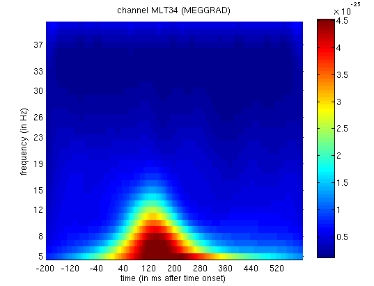
The power spectra for each trial-type can be displayed using the usual Display button and selecting the mtf_cdbspmeeg_SPM_CTF_MEG_example_faces1_3D.mat file. This will produce a plot of power as a function of frequency (y-axis) and time (x-axis) for Channel MLT34. If you use the trial slider to switch between trial(types) 1 and 2, you will see the greater power around 150ms and 10Hz for faces than scrambled faces (click on the magnifying glass icon and on the single channel to get scales for the axes, as in Figure 13. This corresponds to the M170 again.

Total power spectra for faces (left) and scrambled faces (right) for channel MLT34

We can also look at evidence of phase-locking of ongoing oscillatory activity by averaging the phase angle information. We compute the vector mean (by converting the angles to vectors in the complex plane), which yields complex numbers. We can generate two kinds of images from these numbers. The first is an image of the angles, which shows the mean phase of the oscillation (relative to the trial onset) at each time point. The second is an image of the absolute values (also called “Phase-Locking Value”, PLV) which lie between 0 for no phase-locking across trials and 1 for perfect phase-locking.

Select Average Average and select the tph_cdbspmeeg_SPM_CTF_MEG_example_faces1_3D.mat file. Set Compute phase locling value to yes.

Run the batch. The MATLAB window will echo:

  mtph_cdbspmeeg_SPM_CTF_MEG_example_faces1_3D.mat: Number of replications per contrast:
  average faces: 168 trials, average scrambled: 168 trials

and a new file will be created in the MEG directory called mtph_cdbspmeeg_SPM_CTF_MEG_example_faces1_3D.mat.

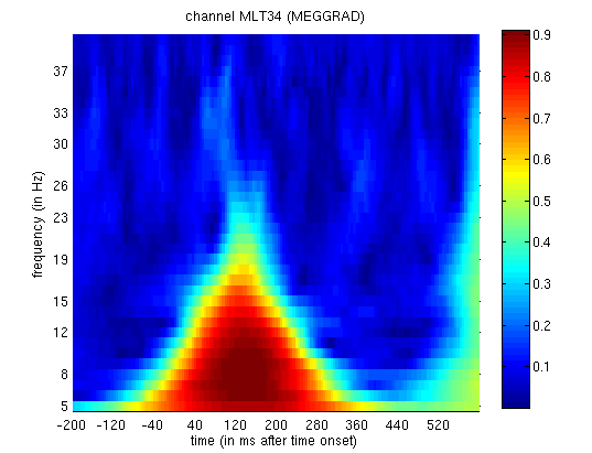
If you now display the file mtph_cdbspmeeg_SPM_CTF_MEG_example_faces1_3D.mat file, you will see PLV as a function of frequency (y-axis) and time (x-axis) for Channel MLT34. Again, if you use the “trial” slider to switch between trial(types) 1 and 2, you will see greater phase-locking around for faces than scrambled faces at lower frequencies, as in Figure 14. Together with the above power analysis, these data suggest that the M170 includes an increase both in power and in phase-locking of ongoing oscillatory activity in the alpha range (Henson et al, 2005b).

Phase-Locking Values for faces (left) and scrambled faces (right) for channel MLT34

2D Time-Frequency SPMs

Analogous to the 3D case, we can also use Random Field Theory to correct for multiple statistical comparisons across the 2-dimensional time-frequency space.

Select Images Convert to images, and select the tf_cdbspmeeg_SPM_CTF_MEG_example_faces1_3D.mat file. Set Mode to time x frequency. Run the batch.

This will create 2 NIfTI files with 2D time-frequency images in each frame with dimensions \(36\times 161\times 1\), as for the example shown in Figure 15. These file can be be found in the tf_cdbspmeeg_SPM_CTF_MEG_example_faces1_3D subfolder. and examined by pressing Display Image in the main SPM window.

If you want to repeat this analysis for other channels the folder with images is in danger of being overwritten every time you do it. To avoid that change the Directory prefix field. You could use a meaningful label like “Left_temporal_”.

3D image for trial 1 within `condition_faces.nii` file. The bottom left section is through frequency (x) and time (y) (the other images are strips because there is only one value in the z dimension, i.e, this is really a 2D image).

As in the 3D case, these images can be further smoothed in time and frequency if desired.

Then as in section on time-domain statistics , we then take these images into an unpaired t-test across trials to compare faces versus scrambled faces. We can then use classical SPM to identify times and frequencies in which a reliable difference occurs, correcting across the multiple comparisons entailed (Kilner et al, 2005).

First create a new directory, eg. mkdir TFstatsPow.

Then press the specify 2nd level button, select two-sample t-test (unpaired t-test), and define the images for group 1 as all the frames in condition_faces.nii (see the previous discussion of statistical analysis for tips on how to select the right frames) and the frames from group 2 as all those in the condition_scrambled.nii file. Finally, specify the new TFstatsPow directory as the output directory.

This would be faster if you saved and could load an SPM job file from the Section on 3D SPMs. In order to just change the input files and output directory.

Then add an Estimate module from the SPM Stats menu, and select the output from the previous factorial design specification stage as the dependency input. Run the batch.

Press Results and define a new T-contrast as \([1\: -1]\). Keep the default contrast options, but threshold at \(p<.05\) FWE corrected for the whole search volume, and then select Time-Frequency for the Data Type. Then press whole brain, and the Graphics window should now look like that in Figure 16.

2D time-frequency SPM T at p<.05. FWE-corrected for the power difference between face and scrambled faces at Channel MLT34.

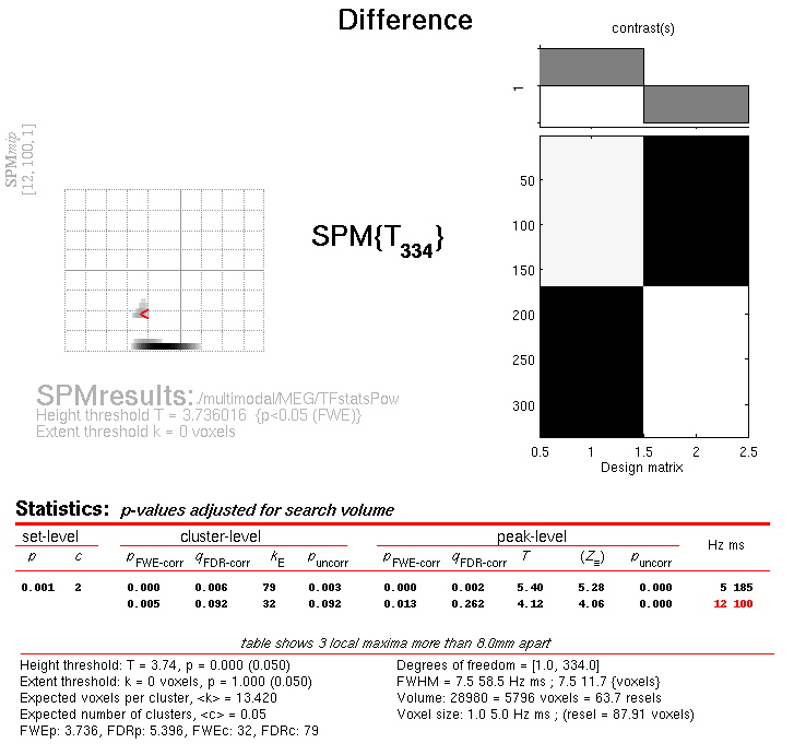
This will list two “regions” within the 2D time-frequency space in which faces produce greater power than scrambled faces, having corrected for multiple T-tests across pixels. The larger one has a maximum at 5 Hz and 185 ms post-stimulus, corresponding to the M170 seen earlier in the averaged files (but now with a statistical test of its significance, in terms of evoked and induced power). The second, smaller region has a maximum at 12 Hz and 100 ms, possibly corresponding to a smaller but earlier effect on the M100 (also sometimes reported, depending on what faces are contrasted with).

“Imaging” reconstruction of total power for each condition

Previously, we localised the differential evoked potential difference in EEG data corresponding to the N170. Here we will localise the total power of faces, and of scrambled faces, ie including potential induced components (see Friston et al, 2006).

Press the 3D source reconstruction button, and press the load button at the top of the new window. Select the cdbspmeeg_SPM_CTF_MEG_example_faces1_3D.mat file and type a label (eg M170) for this analysis.

Press the MRI button, select the smri.img file within the sMRI sub-directory and select the normal mesh.

If you have not used this MRI image for source reconstruction before, this step will take some time while the MRI is segmented and the deformation parameters computed (see above for more details on these files). When meshing has finished, the cortex (blue), inner skull (red) and scalp (orange) meshes will also be shown in the Graphics window with slices from the sMRI image. This makes it possible to verify that the meshes indeed fit the original image well. The field D.inv{1}.mesh will be updated. Press save in top right of window to update the corresponding mat file on disk.

Both the cortical mesh and the skull and scalp meshes are not created directly from the segmented MRI, but rather are determined from template meshes in MNI space via inverse spatial normalisation (Mattout et al, 2007; Henson et al, 2009a).

Press the Co-register button. You will be asked for each of the 3 fiducial points to specify its location on the MRI images. This can be done by selecting a corresponding point from a hard-coded list (select). These points are inverse transformed for each individual image using the same deformation field that is used to create the meshes. The other two options are typing the MNI coordinates for each point (type) or clicking on the corresponding point in the image (click). Here, we will type coordinates based on where the experimenter defined the fiducials on the smri.img. These coordinates can be found in the smri_fid.txt file also provided. So press type and for nas, enter [0 91 -28]; for lpa press type and enter [-72 4 -59]; for rpa press type and enter [71 -6 -62]. Finally, answer no to Use headshape points? (see EEG Section).

To determine the coordinates of MRI fiducials in your subjects’ scans you can open the images using Display Image, identify the anatomical landmarks, locate them with the cursor and copy the coordinates from the coordinates mm box. These can then be saved for future use via the type option.

This stage coregisters the MEG sensor positions with the structural MRI and cortical mesh, via an approximate matching of the fiducials in the two spaces, followed by a more accurate surface-matching routine that fits the head-shape function (measured by Polhemus) to the scalp that was created in the previous meshing stage via segmentation of the MRI. When coregistration has finished, the field D.inv{1}.datareg will be updated. Press save in top right of window to update the corresponding mat file on disk. With the MATLAB Rotation tool on (from the Tools tab in the SPM Graphics window, if not already on), right click near the top image and select Go to X-Z view. This should produce a figure like that in Figure 17, which you can rotate with the mouse to check all sensors. Note that the data are in head space (not MNI space), in this case corresponding to the Polhemus space in which the X and Y dimensions are swapped relative to MNI space.

Graphical output of registration of MEG and sMRI data, showing (upper panel) cortex (blue) and scalp (black) meshes, sensor locations (green), MRI and Polhemus fiducials (cyan/magneta), and headshape (red dots).

Press the Forward Model button. Choose Single Shell (you may also try the other options; see Henson et al, 2009a). A figure will be displaying showing the inner skull surface on which the single shell model is based with the sensors.

Press Invert, select Imaging, select yes to All conditions or trials?, and Standard for the model (i.e, to use defaults; you can customise a number of options if you press Custom instead) (see Friston et al, 2008, for more details about these parameters). There will be lead field computation followed by the actual inversion. A summary plot of the results will be displayed at the end.

You can now explore the results via the 3D reconstruction window. If you type 180 into the box in the bottom right (corresponding to the time in ms) and press mip, you should see several ventral temporal hotspots, as in Figure 18. Note that this localisation is different from the previous EEG localisation because 1) condition 1 now refers to faces, not the difference between faces and scrambled faces, and 2) the results reflect total power (across trials), induced and evoked, rather than purely evoked¹¹. The timecourses come from the peak voxel (with little evidence of a face/scrambled difference for this particular maximum). The red curve shows the condition currently being shown (corresponding to the Condition 1 toggle bar in the reconstruction window); the grey curve(s) will show all other conditions. If you press the condition 1 toggle, it will change to Condition 2, which is the total power for scrambled faces, then press mip again and the display will update (note the colours of the lines have now reversed from before, with red now corresponding to scrambled faces).

Graphic output for MSP-estimated activity at 159ms for faces

If you press movie, you will see the changes in the source strengths over peristimulus time (from the limits 0 to 300ms currently chosen by default).

If you press render it will open a graphical interface that is very useful to explore the data (the buttons are fairly self-explanatory).

You can also explore the other inversion options, like COH and IID, which you will note give more superficial solutions (a known problem with standard minimum norm; see also Friston et al, 2008; Henson et al, 2009a). To do this quickly (without repeating the MRI segmentation, coregistration and forward modelling), press the new button in the reconstruction window, which by default will copy these parts from the previous reconstruction.

In the following we will concentrate on how one prepares this single subject data for subsequent entry into a group analysis.

Press the Window button in the reconstruction window, enter “150 200” as the timewindow of interest and “5 15” as the frequency band of interest (from the SPM time-frequency analysis, at least from one channel). Then choose the induced option. After a delay (as SPM calculates the power across all trials) the Graphics window will show the mean activity for this time/frequency contrast (for faces alone, assuming the condition toggle is showing condition 1).

If you then press Image and select image as the output format, SPM will write 3D NIfTI images corresponding to the above contrast for each condition:

    cdbspmeeg_SPM_CTF_MEG_example_faces1_3D_1_t150_200_f5_15_1.nii
    cdbspmeeg_SPM_CTF_MEG_example_faces1_3D_1_t150_200_f5_15_2.nii

The last number in the file name refers to the condition number; the number following the dataset name refers to the reconstruction number (i.e. the number in red in the reconstruction window, i.e, D.val, here 1).

The smoothed results for Condition 1 will also be displayed in the Graphics window, together with the normalised structural. Note that the solution image is in MNI (normalised) space, because the use of a canonical mesh provides us with a mapping between the cortex mesh in native space and the corresponding MNI space.

You can also of course view the image with the normal SPM “Display:image” option, and locate the coordinates of the “hotspots” in MNI space. Note that these images contain RMS (unsigned) source estimates (see Henson et al, 2007).

If you want to see where activity (in this time/freq contrast) is greater for faces and scrambled faces, you can use SPM ImCalc facility to create a difference image of cdbspmeeg_SPM_CTF_MEG_example_faces1_3D__t150__f5__1.nii - cdbspmeeg_SPM_CTF_MEG_example_faces1_3D__t150__f5__2.nii: you should

see bilateral fusiform. For further discussion of localising a differential effect vs. taking the difference of two localisations, as here, see Henson et al (2007). The above images can then be used at the second level (assuming one also has data from other subjects) to look for effects that are consistent over a group of subjects.

All the steps of 3D source reconstruction can also be carried out via batch by chaining the Head model specification, Source inversion and Inversion results from SPM M/EEG Source reconstruction batch menu.

fMRI analysis

Only the main characteristics of the fMRI analysis are described below; for a more detailed demonstration of fMRI analysis, read previous tutorial chapters describing fMRI analyses.

Toggle the modality from EEG to fMRI, and change directory to the fMRI subdirectory (either in MATLAB, or via the “CD” option in the SPM “Utils” menu)

Preprocessing the fMRI data

Press the Batch button and then:

• Select Spatial Realign' :material-arrow-right-bold:Estimate & Reslicefrom the SPM menu, create two sessions, and select the 390fM*.imgEPI images within the corresponding Session1 / Session 2 subdirectories (you can use the filter^{fM.*where}indicates that the file name must start with 'fM' rather than contain it anywhere). In theResliced imagesoption, chooseMean Image Only`.

• Add Spatial Coregister : Estimate module, and select the smri.img image in the sMRI directory for the Fixed Image and select a Dependency for the Moved Image, which is the Mean image produced by the previous Realign module. For the Other Images, select a Dependency which are the realigned images (two sessions) from Realign (you can use shift-click to seect both).

• Add a Spatial Segment module, and select the smri.img image as Volumes. Set the Save INU corrected option to Save INU corrected. Scroll all the way to the bottom of the options list and set the Deformation fields to Forward.

• Add a Spatial Normalise Normalise: Write module, make a New: Subject, and for the Deformation Feild, select a Dependency of the Segment: Forward Deformations (from the prior segmentation module). For the “Images to Write”, select a Dependency on the Coreg: Estimate: Coregistered Images (which will be all the coregistered EPI images) and Segment: INU Corrected (which will be the bias-corrected structural image). Also, change the Voxel sizes to [3 3 3], to save diskspace.

• Add a Spatial: Smooth module, and for Images to Smooth, select a Dependency on Normalise: Write: Normalised Images (Subj 1).

• Save the batch file (e.g, as batch_fmri_preproc.mat), and then press the button.

These steps will take a while, and SPM will output some postscript files with the movement parameters and the coregistration results (see earlier chapters for further explanation). The result will be a series of 2 sets of 390 swf*.img files that will be the data for the following 1st-level fMRI timeseries analysis.

Statistical analysis of fMRI data

First make a new directory for the stats output, e.g, a Stats subdirectory within the fMRI directory.

Press the batch button and then:

• Select “Stats: fMRI model specification” from the SPM module menu, and select the new Stats subdirectory as the “Directory”.

• Select “Scans” for “Units of design”.

• Enter 2 for the “Interscan interval” (i.e, a 2s TR).

• Create a new session from the “Data & Design” menu. For “Scans”, select all the swf*.img files from the Session1 subdirectory (except the mean). Under “Multiple Conditions”, click “Select File”, and select the trials_ses1.mat file that is provided with these data. (This file just contains the onsets, durations and names of every event within each session.). For “Multiple regressors”, click “Select File”, and select the rp*.txt file that is also in the Session1 subdirectory (created during realignment).

• Repeat the above steps for the second session.

• Under “Basis Functions”, “Canonical HRF” add the “Time and Dispersion” derivatives.

• Then add a “Stats: Model estimation” module, and for the “Select SPM.mat”, choose the “Dependency” of the SPM.mat file from the previous “fMRI model specification” module.

• Add a “Stats: Contrast Manager” module, and for the “Select SPM.mat”, choose the “Dependency” of the SPM.mat file from the previous “Model Estimation module”.

• Under “Contrast Sessions”, create a new F-contrast with a “Name” like faces vs scrambled (all BFs) and then enter [eye(3) -eye(3) zeros(3,6)]. This will produce a 3x12 matrix that picks out the three basis functions per condition (each as a separate row), summing across the two conditions (with zeros for the movement parameter regressors, which are of no interest). Then select “Replicate (average over sessions)”.

• Under “Contrast Sessions”, create a new F-contrast with a “Name” like faces + scrambled vs Baseline (all BFs) and then enter the [eye(3) eye(3) zeros(3,6)]. Again, select “Replicate (average over sessions)”.

• Save the batch file (e.g, as batch_fmri_stats.mat), and then press the “Run” button.

When this has finished, press Results and select the SPM.mat file that should have been created in the new Stats directory. The Contrast Manager window will appear, and you can select the “faces vs scrambled (all BFs)” contrast. Do not mask, keep the title, threshold at \(p<.05\) FWE corrected, use an extent threshold of 60 voxels, and you should get the MIP and table of values (once you have pressed “whole brain”) like that in Figure 19. This shows clusters in bilateral midfusiform (FFA), right occipital (OFA), right superior temporal gyrus/sulcus (STS), in addition to posterior cingulate and anterior medial prefrontal cortex. These clusters show a reliable difference in the evoked BOLD response to faces compared with scrambled faces that can be captured within the “signal space” spanned by the canonical HRF and its temporal and dispersion derivatives. Note that this F-contrast can include regions that show both increased and decreased amplitude of the fitted HRF for faces relative to scrambled faces (though if you plot the “faces vs scrambled” contrast estimates, you will see that the leftmost bar (canonical HRF) is positive for all the clusters, suggesting greater neural activity for faces than scrambled faces (also apparent if you plot the event-related responses)).

There is some agreement between these fMRI effects and the localisation of the differential ERP for faces vs scrambled faces in the EEG data (see earlier section). Note however that the fMRI BOLD response reflects the integrated neural activity over several seconds, so some of the BOLD differences could arise from neural differences outside the 0-600ms epoch localised in the EEG data (there are of course other reasons too for differences in the two localisations; see, eg, Henson et al, under revision).

SPM{F} for faces vs scrambled faces.

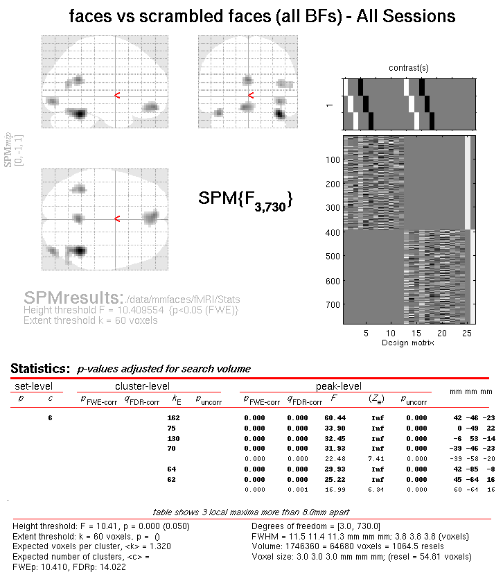
You can also press Results and select the “faces + scrambled vs Baseline (all BFs)” contrast. Using the same threshold of \(p<.05\) FWE corrected, you should see a large swathe of activity over most of the occipital, parietal and motor cortices, reflecting the general visuomotor requirements of the task (relative to interstimulus fixation). The more posterior ventral occipital/temporal BOLD responses are consistent with the MEG localisation of faces (or scrambled faces) versus baseline, though note that the more anterior ventral temporal activity in the MEG localisation is not present in the fMRI data, which suggests (but does not imply) that the MEG localisation may be erroneous.

These contrasts of fMRI data can now be used as spatial priors to aid the localisation of EEG and/or MEG data, as in the next section.

Multimodal fusion

Here, we will illustrate here two types of multimodal integration:

1. “Fusion” of the EEG and MEG data (Henson et al, 2009b),

2. Use of the fMRI data as spatial priors on the MEG/EEG data (Henson et al, in press).

EEG and MEG fusion

Make a new directory called “Fused’, and change into it.

Merging the EEG and MEG datafiles

The first step is to combine the MEG and EEG data into a single SPM file. We will use the (weighted) averaged files for each modality.

Select Preprocessing Fuse', and select thewmcdbspmeeg_SPM_CTF_MEG_example_faces1_3D.matin the MEG directory and thewmaceMdspmeeg_faces_run1.matin the EEG directory. This will create a new file calleduwmcdbspmeeg_SPM_CTF_MEG_example_faces1_3D.mat` in the MEG directory. Note that the two files need to have the same number of trials, conditions, samples, etc. Display the new file, and you will see the EEG and MEG data within their respective tabs.

We have to do one extra bit of “preparation” for the EEG data. Because in general, one might want to merge more than one EEG file, integrating all their locations could be tricky. So the simple answer is to clear all locations and force the user to re-specify them. So (as in earlier EEG section), select Convert Prepare and open the uwmcdbspmeeg_SPM_CTF_MEG_example_faces1_3D.mat file. Then in the Sensors submenu, choose Load EEG sensors Convert locations file, and select the electrode_locations_and_headshape.sfp file (in the original EEG directory). Then from the 2D projection submenu select Project 3D (EEG). A 2D channel layout will appear in the Graphics window. Select Apply from 2D Projection and Save from File submenu.

3D fused “imaging” reconstruction

Now we can demonstrate simultaneous reconstruction of the MEG and EEG data, as described in Henson et al (2009b). This essentially involves scaling each type of data and gain matrix, concatenating them, and inverting using the normal methods, but with separate sensor error covariance terms for each modality.

• Press the 3D source reconstruction button, and load the uwmcdbspmeeg_SPM_CTF_MEG_example_faces1_3D.mat file. Type a label (eg “N/M170”).

• Press the MRI button, select the smri.img file within the sMRI sub-directory, and select normal for the cortical mesh. Because this MRI was normalised previously, this step should not take long, finishing with display of the cortex (blue), inner skull (red), outer skull (orange) and scalp (pink) meshes.

• Press the Co-register button. Press type and for nas, enter [0 91 -28] for lpa press type and enter [-72 4 -59] for rpa press type and enter [71 -6 -62]. Finally, answer no to Use headshape points?. Then select either EEG or MEG to display corresponding data registration. Note that the MEG data will have been coregistered to the EEG data in the headspace. If you want to display the other modality afterwards, just press the display button below the Co-register button.

• Press Forward Model, and select EEG BEM for the EEG and Single Shell for the MEG. Then select either EEG or MEG to display the corresponding forward model. (If you want to display the other modality afterwards, just press the display button below the Forward Model button). In the Graphics window the meshes will be displayed with the sensors marked with green asterisks.

• Press save to save progress.

• Press Invert, select Imaging. Because the fMRI data (see below) already come from a contrast of faces versus scrambled faces, we will only invert the differential ERP/ERFs. So press no to the question about invert all conditions or trials, press yes to invert the Difference (between faces and scrambled) but no to invert the Mean (of faces and scrambled versus baseline).

Then press Standard to use the default inversion settings (MSP), and then to select both the EEG and MEG modalities in the new Select modalities window, in order to fuse them (simultaneously invert both).

Lead fields will first be computed for all the mesh vertices and saved in the file SPMgainmatrix_uwmcdbspmeeg_SPM_CTF_MEG_example_faces1_3D_1.mat. This will take some time. Then the actual MSP algorithm will run and the summary of the solution will be displayed in the Graphics window.

• Press save to save the results. You can now explore the results via the 3D reconstruction window. If you type 180 into the box in the bottom right (corresponding to the time in ms) and press mip, you should see an output similar to Figure 20.

Graphical output of an MSP estimation of the differential evoked response between faces and scrambled faces at 180ms, after fusing both EEG and MEG data.

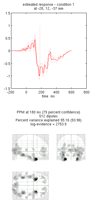
Note that because we have inverted only the differential ERP/ERF, these results cannot be compared directly to the unimodal inversions in the previous sections of this chapter. For a fairer comparison:

• Press the new button and type “N170” as the label, press Invert again (note that all forward models are copied by default from the first inversion) and select the same options as above, except that when asked Select modalities, select just EEG. This should produce the results in

Figure 21. Notice the more posterior maxima.

Graphical output of an MSP estimation of the differential evoked response between faces and scrambled faces at 180ms, after inverting just EEG data.

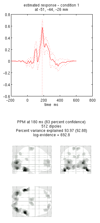
• Press the new button and type “M170” as the label, press Invert again and select the same options as above, except that when asked Select modalities, select just MEG this time. This should produce the results in Figure 22. Notice the more anterior and medial activity.

Graphical output of an MSP estimation of the differential evoked response between faces and scrambled faces at 180ms, after inverting just MEG data.

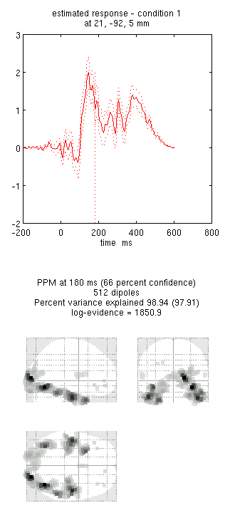
By comparing these figures, you can see that the multimodal fused inversion (first inversion) combines aspects of both the unimodal inversions. Unfortunately one cannot simply compare the multi-modal vs uni-modal reconstructions via the log-evidence, because the data differs in each case (rather, one could use an estimate of the conditional precision of the sources, as in Henson et al, 2009b). With multiple subjects though, one could compare statistics across subjects using either multimodal or unimodal inversions.

EEG, MEG and fMRI fusion

Now we can examine the effects of using the fMRI data as spatial priors on the sources (Henson et al, in press). But first we need to create an 3D volumetric image of the clusters that we wish to use as spatial priors. These clusters can be defined by thresholding an SPM for a given fMRI contrast: here we will use the contrast of faces versus scrambled faces (using all three basis functions). So press Results and select the SPM.mat file from the fMRI/Stats directory. Select the previous faces vs scrambled F-contrast, do not mask or change title, use FWE correction at 0.05 and a 60-voxel extent to reproduce the SPM{F} shown in Figure 19 (if you are still in SPM’s “EEG” mode, you will also be asked the type of images, for which you reply Volumetric 2D/3D).

Now press the save button in the Interactive window and enter a filename like FacesVsScrambled_FWE05_60. This will produce a 3D image (which you can display as normal) in which all subthreshold voxels are set to zero (ie, where only 6 clusters containing non-zero voxel values are left).

Now we can use this cluster image in a new inversion:

• Press the new button to create a fourth inversion, and type “N/M170+fMRI” as the label.

• Press Invert, select Imaging, press no for all conditions or trials, and select only the Difference (not Mean), as before ...

• ... but this time, press Custom rather than Standard to get more flexibility in the inversion settings. Select GS for the type of inversion (the default MSP with a Greedy Search), enter default time window of “-200 to 600”, yes to a Hanning window, 0 for the highpass and 48 for the lowpass, and then press yes to the question of Source priors?...

• ... select the FacesVsScrambled_FWE05_60.img file in the “fMRI/Stats” directory, and select MNI for the Image space (because the fMRI images were spatially normalised).

• Say No to Restrict solutions, and then select both the EEG and MEG modalities in the Select modalities window, in order to fuse them (together with the fMRI priors).

Note that, once the inversion has finished, a new image will be created (in the “fMRI/Stats” directory) called cluster_FacesVsScrambled_FWE05_60.img, which contains the six binary priors, as will a GIfTI version called priors_uwmcdbspmeeg_SPM_CTF_MEG_example_faces1_3D_4.func.gii. If you want to display each spatial prior on the cortical mesh, first make sure you save the current reconstruction, and then type in the MATLAB window:

    D = spm_eeg_load('uwmcdbspmeeg_SPM_CTF_MEG_example_faces1_3D.mat');
    val = 4;    % Fourth inversion; assuming you have followed the above steps
    G = gifti(D.inv{val}.mesh.tess_mni);
    P = gifti(D.inv{val}.inverse.fmri.texture);
    for i=1:size(P.cdata,2);
      figure, plot(G,P,i);
    end

Finally, a new MATLAB file called priors_uwmcdbspmeeg_SPM_CTF_MEG_example_faces1_3D_4.mat will also be saved to the current directory, which contains the information necessary to construct the covariance components for subsequent inversion. So if you want to use these fMRI priors in another inversion, next time you are prompted for the “Source priors?”, rather than selecting an image (“img” file) as we did above, you can select this “mat” file, so SPM will not need to recreate the covariance matrices from the image file, but can use the covariance matrices directly.

• Again, type 180 into the box in the bottom right and press “mip”. This should produce the output in Figure 23. Notice how the more posterior midfusion clusters (particularly on the left) have become stronger (where there were fMRI priors). (Note also that fMRI priors have generally been found to have a greater effect on IID or COH inversions, given the implicit flexibility of MSP priors, Henson et al, in press).

Graphical output of an MSP estimation of the differential evoked response between faces and scrambled faces at 180ms, after fusing EEG, MEG and fMRI data.

---

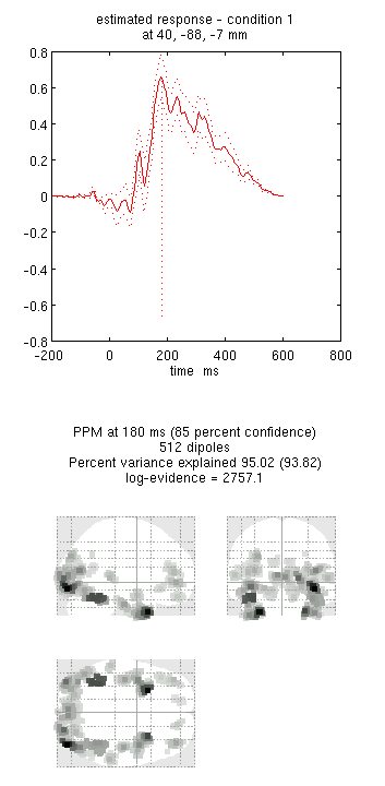
1. Re-referencing EEG to the mean over EEG channels is important for source localisation. Note also that if some channels are subsequently marked “bad” (see later), one should re-reference again, because bad channels are ignored in any localisation. ↩

2. You might need to change the full path to this text file inside the single quotes, depending on your current directory and the directory of the original data. ↩

3. When there are approximately equal numbers of trials in each condition, as here, it is probably safer to compute weights across all conditions, so as not to introduce artifactual differences between conditions. However, if one condition has fewer trials than the others, it is likely to be safer to estimate the weights separately for each condition, otherwise evoked responses in the rarer condition will be downweighted so as to become more similar to the more common condition(s). ↩

4. Note that the 2D location in sensor space for EEG will depend on the choice of montage. ↩

5. Note that we can use the default “nonsphericity” selections, i.e, that the two trial-types may have different variances, but are uncorrelated. ↩

6. The former likely corresponds to the “N170”, while the latter likely corresponds to the “VPP”, which may be two signs of the same effect, though of course these effects depend on the choice of reference. ↩

7. Note that no new M/EEG files are created during the 3D reconstruction; rather, each step involves updating of the cell-array field D.inv, which will have one entry per analysis performed on that dataset (e.g, D.inv{1} in this case). ↩

8. Alternatively, you could correct by 1 refresh, to match the delay in the EEG data. ↩

9. You can of course obtain time-frequency plots for every channel, but it will take much longer (and result in a large file). ↩

10. For example, for 5Hz, one would need at least N/2 x 1000ms/5, where N is the order of the Morlet wavelets (i.e, number of cycles per Gaussian window), e.g, 600ms for a 6th-order wavelet. ↩

11. Though in reality, most of the power is low-frequency and evoked ↩