DCM for Cross Spectral Densities: Anaesthesia Depth in Rodent Data
Overview
This chapter describes the analysis of a 2-channel Local Field Potential (LFPs) data set using dynamic causal modelling. The LFPs were recorded from a single rodent using intracranial electrodes (Moran, Stephan, Jung, et al. 2009). We thank Marc Tittgemeyer for providing us with this data. The theory behind DCM for cross spectral densities (DCM-CSD) is described in (Friston et al. 2012). This DCM is a generalization of DCM for Steady State Responses to the complex domain (Moran, Stephan, Seidenbecher, et al. 2009). The generative model now reports coherence and signal covariance as well as complex spectral densities (from which the former are derived).
We measured local field potentials from primary (A1) and secondary auditory (A2) cortex in a rodent following the application of four different doses of the anaesthetic agent Isoflurane; 1.4, 1.8, 2.4 and 2.8%. The rodent was presented with a white noise auditory input for several minutes at each anaesthetised level and time series recordings were obtained for the entire epoch. We performed a DCM analysis to ask whether changes in neuronal activity induced by increasing levels of Isoflurane are best accounted for by either extrinsic or intrinsic changes in connectivity.
We demonstrate in this chapter the consistency of the model comparison and conditional parameter estimates across different population models. In particular we modeled the CSD as the output of a two region network comprising either “CMC” or “NMDA” – type neural mass models.
The CMC-type neural mass model comprises four subpopulations. It is a
refinement of the Jansen and Rit convolution models that explicitly
accommodates the neuronal sources of forward and backward connections in
cortical hierarchies (Bastos et al. 2012). These are distinct
superficial and deep pyramidal cell populations respectively that,
crucially, may exhibit different spectral outputs. The CMC thus utilizes
different types of subpopulations as the source of forward and backward
connections. For the forward connections superficial pyramidal cells
excite stellate cells and deep pyramidal neurons, while the backward
connections inhibit superficial pyramidal cells and inhibitory
interneurons (see spm_fx_cmc). From the graphical user interface trial
specific effects can be selected for extrinsic connections or intrinsic
connections, for the CMC case the intrinsic connection that is modulated
is an inhibitory gain parameter on superficial pyramidal cells. The
smaller this value, the greater the gain on this cell population due to
the modulation.
The NMDA model uses an architecture comprising three subpopulations,
each assigned to a particular cortical layer. An inhibitory interneuron
subpopulation occupies agranular layers. This receives inputs from
excitatory pyramidal cells, also in agranular layers which are, in turn,
driven by excitatory spiny cells in the granular layer; layer IV. These
three subpopulations are connected with intrinsic coupling parameters
(which can be found in spm_fx_mnn_nmda). Forward connections
correspond to afferent pyramidal axons and synapse on layer IV stellate
cells, while backward afferents impinge upon pyramidal and inhibitory
interneurons outside of layer IV. Lateral, inter-hemispheric connections
are modelled with a postsynaptic response that is elicited in all
layers. The model employs Morris Lecar-type differential equations to
describe the time evolution of a neuronal ensemble. In this model, cells
possess AMPA, GABAA, and NMDA-like receptor dynamics, with appropriate
ion-channel time constants and a voltage dependent switch for the NMDA
channel (Moran et al. 2011). From the graphical user interface trial
specific effects can be selected for extrinsic connections or intrinsic
connections, for the NMDA case the intrinsic connection that is
modulated is an excitatory connection operating on all intrinsic
excitatory connections. The greater this value, the greater the
excitatory effect due to the modulation.
Main Results
Using Bayesian model comparison we found very strong evidence (Bayes Factor\(_{1,2}\) \(>\) 100) in favour of a model comprising a network of two neural masses connected by forward and backward connections from A1 to A2 and A2 to A1, where the effect of anesthetic was best explained by changes in intrinsic connections (model 2). This outperformed a model comprising the same two neural masses with the same extrinsic connections but where the effect of isoflurane was expressed as a modulatory (B) effect on extrinsic connections – between regions (model 1). This result was obtained for both types of neural mass models used.
Using the Graphical User Interface to Obtain those Results
In what follows, these results will be recreated step-by-step using
SPM12. To proceed with the data analysis, first download the data set
from the SPM website1. The data comprises a data file called
dLFP_white_noise_r24_anaes.dat and its corresponding MAT-file
dLFP_white_noise_r24_anaes.mat. This has been converted from ASCII
data using spm_lfp_txt2mat_anaes.m also on the website and
subsequently downsampled to 125 Hz. The conversion script can be altered
to suit your own conditions/sampling parameters.
The data
-
To check data parameters after conversion using ASCII files: in the SPM M/EEG GUI press Display/M/EEG.
-
In our data set we can see there are five trials: four depths of anaesthetic: Iso14, Iso18, Iso24 and Iso28 and one awake trial awake.
-
We are going to employ a 5 sec window of data (without ripples) for the DCM – this data is from 25000 to 30000 ms.
-
We are now ready to begin the DCM analysis. To open the DCM GUI press DCM in the SPM M/EEG GUI.
Dynamic Causal Modelling of Cross Spectral Densities
-
Before you begin any DCM analysis you must decide on three things: the data feature from your time series, the model you wish to use and the hypothesis you wish to test.
-
For our long time series we will examine the steady state and so in the top panel of the DCM GUI select CSD in the data drop-down menu.
-
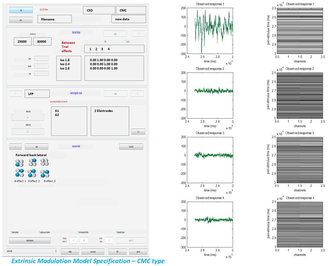
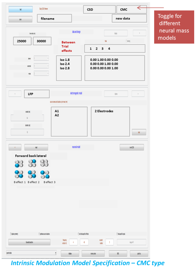
Next in the second drop down menu we select our model. For our first analysis we select the CMC model (we can toggle this button to select other types of neural masses later.) Then we are ready to load our data: press new data and select the file
dLFP_white_noise_r24_anaes.mat. -
Press the red arrow to move forward.
-
The second panel allows you to specify the data and design. We will use 5 seconds of data towards the end of the recording for our analysis. To specify this timing enter 25000 and 30000 in the time window.
-
Next we select the detrending parameters which we set to 1 for detrend, 1 for subsample (as the data has already been downsampled) and 2 for the modes (in this case this is the same as the number of channels) using the drop down menus.
-
We can then specify which trials we want to use. Since we are interested in the anaesthetized trials we enter [1 2 3 4] under the trials label and Iso 1.8 Iso 2.4 Iso 2.8 are our three effects in the “between trial effects” panel. Next we specify the design matrix. This is entered numerically in the large panel. Since we have 4 trials and 3 between trial effects (one less) we enter a matrix with rows: [0 1 0 0] (row 1), [0 0 1 0] (row 2) and [0 0 0 1] (row 3). This will allow us to examine “main effect” differences between the four conditions.
-
Press the red arrow to move forward.
-
The third panel contains the spec for the electromagnetic model. This is very simple for local field potential recordings. In the drop down menu select LFP. In the source names panel, enter A1 and A2. You are finished.
-
Press the red arrow to move forward.
-
At this point all that is left to specify is the neuronal model in terms of its connectivity. We wish to compare two different models so we can save the specifications so far using the save button and reload the above specs for both neuronal models.
-
To specify the neuronal model, load the DCM (that you just saved) as it has been so far specified.
-
Our first model is the extrinsic modulation model.
-
So we specify forward connections from A1 to A2 and backward connections from A2 to A1.
-
We finally specify the B effects where we enter our hypothesis of connectivity changes between trial 1 (Iso1.4%) trial 2 (Iso1.8%) trial 3 (Iso2.4%) and trial 4 (Iso2.8%). Changes will be specified relative to trial 1.
-
We enter the off diagonal entries to correspond to forward connections (as entered in the above panel) to specify extrinsic connectivity changes between A1 and A2 due to (anaesthetic) condition.
-
Finally we enter the frequencies we are interested in: we will fit frequencies from 4 to 48 Hz.
-
To invert the model press the “invert DCM” button.
-
Repeat the procedure after loading the saved specs and repeating for new neuronal models as per figure 1.2. Here we enter our alternative hypothesis (model 2) and fit a second model where instead of extrinsic connectivity changes, the isoflurane related-changes are generated by connectivity differences within a region – we call this the intrinsic modulation model.
-
This is specified by selecting the diagonal elements of the B-matrices.
Comparing models using Bayesian Model Selection
-
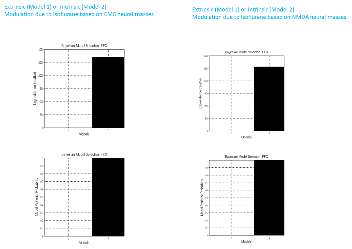
Once both models have run, we compare their evidences to find the best or winning model. To do this press the BMS button. This will open the SPM batch tool for model selection. Specify a directory to write the output file to. For the Inference method select Fixed effects (see (Stephan et al. 2009) for additional explanations). Then click on Data and in the box below click on New: Subject. Click on Subject and in the box below on New: Session. Click on models and in the selection window that comes up select the DCM mat files for all the models (remember the order in which you select the files as this is necessary for interpreting the results). Then run the model comparison by pressing the green Run button. You will see at the top, a bar plot of the log-model evidences for all models (Figure 1.3). The bottom panel displays the conditional probability, for each model assuming equal priors on model space. By convention, a model can be said to be the best among a selection of other models, with strong evidence, if its log-model evidence exceeds all other log-model evidences by at least 3. You can also compare model evidences manually if you load the DCMs into MATLAB ‘s workspace and find the evidence in the structure under DCM.F.
-
For our example we see that there is strong model in favor of model 2 (log Bayes Factor >2500); ie. Isoflorane effects are better explained by a modulation of intrinsic connections.
-
We repeated the steps above and inverted two models (again with either extrinsic or intrinsic modulations) using the CMC and the NMDA neural masses also. These yielded similar results in favor of model 2 – an intrinsic connectivity effect.
-
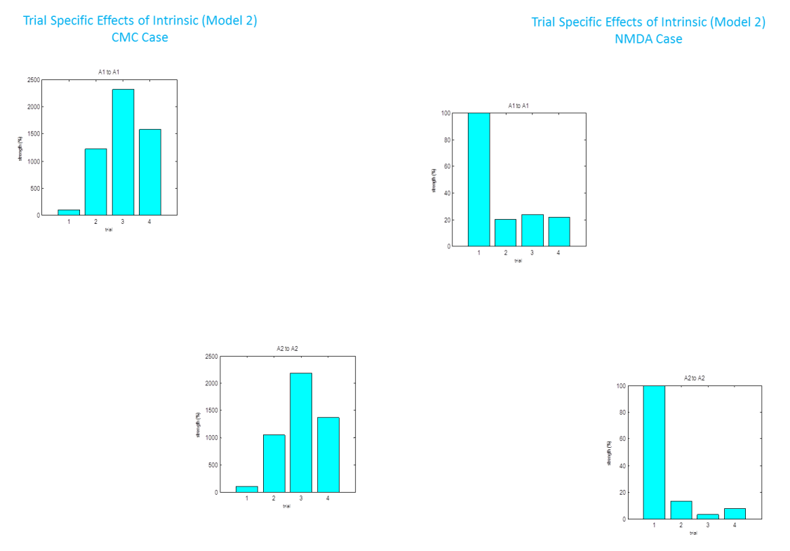
Once inverted a results tab appears which allows you to view the fits to the spectral data, posterior parameter estimates, coherence and covariance (in channel and source space) and the transfer functions between regions. You can also examine the direction of the modulating “B” effects under “trial specific effects”.
-
From our winning CMC model we examined the trial specific effects and found a large increase for trial 2 relative to trial 1 in A1 (top left panel). Remember for the CMC case this represents a decreases in pyramidal cell gain – and so is a net inhibitory effect, consistent with the physiological effects of Isoflurane. The effect was even larger for trial 3 compared to trial 1 and decreased to a lower level for trial 4 (as reported in (Moran et al. 2007)). The effects were similar in A2 (bottom right panel). We found a very similar trial specific effect in the NMDA case, but here the parameter decreases as it represents a positive modulation of an excitatory connection. In other words the effect of increasing isoflurane levels inhibitory in a non-linear fashion (saturating at a level of 2.4%; trial 3).
-
Anaesthesia Depth in Rodent Dataset: http://www.fil.ion.ucl.ac.uk/spm/data/dcm_csd/ ↩