Multimodal, Multisubject data fusion
Time-Frequency Analysis (Evoked and Induced power)
The above statistical test only identifies significant evoked effects (i.e., that are phase-locked across trials) within one individual. We can also look at induced as well as evoked energy by performing a time-frequency analysis before averaging over trials. Here we will use Morlet wavelets to decompose each trial into power and phase across peristimulus time and frequency. We will then average the power estimate across trials and across channels, to create a 2D time-frequency image, which we can then test for reliability, but now across subjects rather than across trials. This is the second fork in the preprocessing pipeline.
Wavelet estimation
The first module to be added to the pipeline is the “Time-Frequency
Analysis” under “SPM – M/EEG – Time-frequency”. Highlight “File Name”,
choose “Specify” box, and select the file Mcbdspmeeg_run_01_sss.mat.
This file has not yet been cropped because we need the 400ms buffer to
reliably estimate the lower-frequency wavelets (in fact, for a 5-th
order 6Hz wavelet, one needs 2.5 periods = 2.5\(\times\)133ms
\(\sim\)400ms to reliably estimate power at the central
timepoint). Note that this file does not have artifacts removed, but
most of these identified for the evoked analysis above are blinks, which
are typically below \(\sim\)3Hz, i.e., below the lowest frequency
of interest here.
Next, ensure “channel selection” is set to “all”. Then highlight the
“Frequencies of interest”, click “Specify” and enter 6:40 (which will
estimate frequencies from 6 to 40Hz in steps of 1Hz). Then highlight
“Spectral estimation” and select “Morlet wavelet transform”. Then
highlight “Number of wavelet cycles” and “Specify” this as 5. The
fixed time window length should be set at 0 as default. To reduce the
size of the file, we will also subsample in time by a factor of 5 (i.e.,
every 25ms, given the additional downsampling to 5ms done earlier in
preprocessing). Do this by selecting “subsample” and “Specify” as 5.
Finally, select “Yes” for “Save phase”. This will produce two files, one
for power (prefixed with tf) and one for phase (prefixed with tph).
Crop
Once we have estimated power and phase at every peristimulus timepoint,
we can cut the 400ms buffer. So add the “SPM – M/EEG – Preprocessing
– Crop” module (like for the evoked analysis). This module will have to
be added twice though, once for power and once for phase. For the first
module, select the power file as the dependency, and enter [-100 800]
as the timewindow. Then select “replicate module”, and change only the
input dependency to the phase file.
Average
As with cropping, we now need to add two averaging modules, one with
dependency on the power file from the Crop step, and the other with
dependency on the phase file from the Crop step. For the power
averaging, choose straight averaging. For the phase averaging however,
we need to additionally select “Yes” to the “Compute phase-locking
value”. This corresponds to “circular” averaging, because phase is an
imaginary number. This produces a quantity called the phase-locking
value (PLV). The prefix will be m in both cases.
Baseline rescaling
To baseline correct time-frequency data, we need to select the
“Time-Frequency Rescale” option from the “Time-Frequency” menu (note:
not the “Baseline Correction” module from the “Preprocessing” menu).
There are several options to baseline-correct time-frequency data. For
the power, it also helps to scale the data with a log transform, because
changes at high-frequency tend to be much smaller than changes at lower
frequencies. We will therefore use the log-ratio (“LogR”) option, where
all power values at a given frequency are divided by the mean power from
-100 to 0ms at that frequency, and the log taken (which is equivalent to
subtracting the log of the baseline power). So select the power file
output from the previous phase as the dependency, select the log ratio
option, and enter the baseline time window as -100 0. The output file
prefix will be r. We won’t bother to baseline-correct the phase-data.
Contrasting conditions
Finally, like with the evoked fork, we can take contrasts of our
trial-averaged data, e.g., to create a time-frequency image of the
difference in power, or in PLV, between faces and scrambled faces.
Create two “SPM – M/EEG – Average – Contrast over epochs” modules,
one with the average power file as input, and one with the averaged
phase (PLV) file as input. You can then select “New Contrast” and enter
contrasts like [0.5 0.5 -1] (for faces vs scrambled; see earlier) and
[1 -1 0] (for famous vs unfamiliar). The resulting output file is
prepended with w.
As before, if you want to save file-space, you can add further “Delete” modules, since we will not need many of the intermediate files. The only files we need to keep are the averaged power and phase files (since these are used to create time-frequency images below) and the contrasted versions (for visual inspection of effects within each subject).
Save batch and review.
You can now save this time-frequency batch file (it should look like the
batch_preproc_meeg_tf_job.m file in the SPM12batch FTP directory).
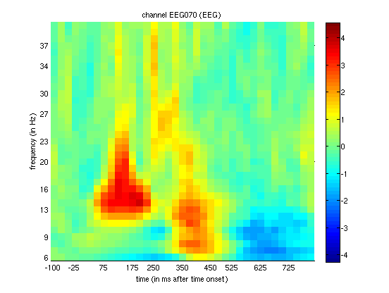
Once you have run it, you can then review the contrast files, e.g, for
power (wmprtf_Mcbdspmeeg_run_01_sss.mat) or phase
(wmptph_Mcbdspmeeg_run_01_sss.mat). When displaying the power for the
EEG data, if you magnify Channel 70 (right posterior, as in
Figure 1.3), you should see something like
that in Figure 1.8. The increase in power from 13 to
16Hz between 75 and 200ms is most likely the evoked energy corresponding
to the N170 in Figure 1.3, but additional power changes can
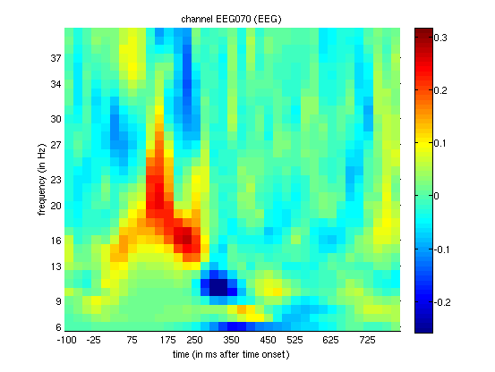
be seen that may not be so phase-locked (i.e. induced). This is
supported by looking at the difference in PLV for that channel
(Figure 1.9), where faces increase
phase-locking relative to scrambled faces in a similar time-frequency
window (suggesting a change in phase of ongoing alpha oscillations, as
well as their power).
Creating 2D time-frequency images
Later we will repeat the above steps for every subject, and create a
statistical parametric map of power changes across subjects, in order to
localise face-induced power changes in frequency and time. This requires
that we create 2D images, one per condition (per subject). Select the
“convert2images” option and select the baseline-rescaled, trial-averaged
power file as the dependency from the stage above. Select the mode “time
x frequency”. Note that this implicitly means averaging across all
channels. Next select channel selection by type. Here, choose EEG for
“Channel selection” and define the prefix as eeg_img_pow. (Of course,
this module can be repeated for MEGMAG and MEGPLANAR sensors if wanted.)
You can save this batch, run it, and display the images output if you
like (the FTP batch is called batch_preproc_meeg_tf_images_job.m).
Creating a script for analysis across subjects.
Now that we have created pipelines for various steps of preprocessing
one subject, including the two forks for evoked and time-frequency
analyses, we want to run these on the remaining 15 subjects. For this, a
bit of MATLAB knowledge is required to call these pipelines within a
for (or parfor) loop across subjects. Below is an example from the
master_script.m:
for s = 1:nsub

    %% Change to subject's directory
    swd = fullfile(outpth,subdir{s},'MEEG');
    cd(swd);

    %% Convert & epoch, prepare, downsample, baseline-correct each run
    jobfile = {fullfile(scrpth,'batch_preproc_meeg_convert_job.m')};
    jobs    = repmat(jobfile, 1, nrun);
    n = 1;
    inputs  = cell(nrun*3, 1);
    for r = 1:nrun
        inputs{n  ,1} = cellstr(fullfile(rawpth,subdir{s},'MEEG',sprintf('run_%02d_sss.fif',r)));
        inputs{n+1,1} = cellstr(fullfile(rawpth,subdir{s},'MEEG','Trials',sprintf('run_%02d_trldef.mat',r)));
        inputs{n+2,1} = cellstr(fullfile(rawpth,subdir{s},'MEEG','bad_channels.mat'));
        n = n + 3;
    end
    spm_jobman('serial' , jobs, '', inputs{:});

    %% Concatenate runs and montage (reref EEG)
    jobfile = {fullfile(scrpth,'batch_preproc_meeg_merge_job.m')};
    inputs  = cell(3, 1);
    inputs{1} = cellstr(spm_select('FPList',fullfile(outpth,subdir{s},'MEEG'),'^bdspmeeg.*\.mat$'));
    inputs{2} = cellstr(spm_select('FPList',fullfile(outpth,subdir{s},'MEEG'),'^bdspmeeg.*\.mat$'));  % (For deletion)
    spm_jobman('serial', jobfile, '', inputs{:});

    %% Fork 1. For ERP/ERF: crop to -100 to +800, detect artifacts (blinks) by thresholding EOG, combine planar grads, average over trials and create contrasts of conditions
    jobfile = {fullfile(scrpth,'batch_preproc_meeg_erp_job.m')};
    inputs  = cell(1);
    inputs{1} = cellstr(spm_select('FPList',fullfile(outpth,subdir{s},'MEEG'),'^Mcbdspmeeg.*\.mat$'));
    spm_jobman('serial', jobfile, '', inputs{:})

    %% Write out scalp-time images
    if strcmp(subdir{s},'Sub15')
    jobfile = {fullfile(scrpth,'batch_preproc_meeg_erp_images_job.m')};
    inputs  = cell(3,1);
    inputs{1} = cellstr(spm_select('FPList',fullfile(outpth,subdir{s},'MEEG'),'^PapMcbdspmeeg.*\.mat$'));
    inputs{2} = cellstr(spm_select('FPList',fullfile(outpth,subdir{s},'MEEG'),'^PapMcbdspmeeg.*\.mat$'));
    inputs{3} = cellstr(spm_select('FPList',fullfile(outpth,subdir{s},'MEEG'),'^PapMcbdspmeeg.*\.mat$'));
    spm_jobman('serial', jobfile, '', inputs{:});
    end

    %% Fork 2. For Time-freq: Morlet wavelet transform, crop, average, baseline-correct (power) and contrast
    jobfile = {fullfile(scrpth,'batch_preproc_meeg_tf_job.m')};
    inputs  = cell(1);
    inputs{1} = cellstr(spm_select('FPList',fullfile(outpth,subdir{s},'MEEG'),'^Mcbdspmeeg.*\.mat$'));
    spm_jobman('serial', jobfile, '', inputs{:});

    %% Write out power and phase images for each modality
    jobfile = {fullfile(scrpth,'batch_preproc_meeg_tf_images_job.m')};
    inputs  = cell(6,1);
    inputs{1} = cellstr(spm_select('FPList',fullfile(outpth,subdir{s},'MEEG'),'^mprtf_Mcbdspmeeg.*\.mat$'));
    inputs{2} = cellstr(spm_select('FPList',fullfile(outpth,subdir{s},'MEEG'),'^mprtf_Mcbdspmeeg.*\.mat$'));
    inputs{3} = cellstr(spm_select('FPList',fullfile(outpth,subdir{s},'MEEG'),'^mprtf_Mcbdspmeeg.*\.mat$'));
    inputs{4} = cellstr(spm_select('FPList',fullfile(outpth,subdir{s},'MEEG'),'^mptph_Mcbdspmeeg.*\.mat$'));
    inputs{5} = cellstr(spm_select('FPList',fullfile(outpth,subdir{s},'MEEG'),'^mptph_Mcbdspmeeg.*\.mat$'));
    inputs{6} = cellstr(spm_select('FPList',fullfile(outpth,subdir{s},'MEEG'),'^mptph_Mcbdspmeeg.*\.mat'));
    spm_jobman('serial', jobfile, '', inputs{:});

end
Time-frequency Stats across Subjects
We can now enter the frequency-time power images (one per condition per subject) into a group (2nd-level) analysis that corresponds to repeated-measures ANOVA. Note that one difference from the ANOVA used for scalp-time analysis across trials within one subject above is that we now have 3 observations (conditions) from each subject, so need to correct for the potential correlation (nonsphericity) of the error induced by these repeated measurements. We can also add another 16 columns into our GLM that serve to remove between-subject variance (which we don’t care about), improving the sensitivity of contrasts of our conditions of interest.
The first thing is to specify the output directory where the SPM stats
files will be saved. Because this is now an analysis across subjects, we
can create a directory above Sub15 in the directory tree. So create a
new top-level directory called, for example, “MEEG” (because later we
will have group stats for the fMRI data and source-reconstructed MEEG
data too), then a sub-directory within it called TFStats, and then a
further sub-directory called PowStats and a further sub-directory
called eeg (and potentially two more called mag and grd if you
want to examine other sensor-types too).
Model Specification, Estimation and Contrasts
To create this repeated-measures ANOVA, open a new batch and select
“Factorial design specification” under “Stats” on the “SPM” toolbar.
Then select this new MEEGTFStats/PowStats/eeg directory.
Highlight “Design” and from the current item window, select “One-way
ANOVA –within subject” (somewhat confusingly, this is not an analysis
within one subject, as above, but an analysis in which multiple measures
come from “within” each subject!). Highlight “Subjects” and create a
“New:subject”. In the “scans” field, you can now select the 3 power
images for the first subject (which should have been created in the
Sub01/MEEG/eeg_img_pow_mprtf_Mcbdspmeeg_run_01_sss directory if you
ran the script above), and enter the “Conditions” as [1 2 3]. It is
important for the contrasts below that you select the files in the order
Famous-Unfamiliar-Scrambled (or if not, that you change the order of 1-3
in the Conditions vector, such that Condition 1 is Famous, Condition 2
Unfamiliar, etc.). You can then select “Replicate: Subject” under the
“Subjects” item, keeping the “Conditions” unchanged, but changing the
“Scans” to those in
Sub02/MEEG/eeg_img_pow_mprtf_Mcbdspmeeg_run_01_sss. You can then
repeat these steps for the remaining subjects. Or if you prefer (because
this is a pain to do via the GUI!), you can create 16 blank “Subject”
items, save the batch script, and then populate the “Scans” field (and
Conditions field) via a MATLAB script (see below). Finally, set the
variance to “Unequal” and the “Independence” to “No” (to model the error
correlation, i.e., nonsphericity, mentioned above). Keep all the
remaining defaults.
The next step is to add a module for model estimation from the “Stats” option and define the file name as being dependent on the results of the factorial design specification output. For “write residuals”, keep “no”. Select classical statistics.
The final step is to add a module for creating contrasts. Define the
file name as dependent on the model estimation. The first contrast will
be a generic one that tests whether significant variance is captured by
the first 3 regressors. This corresponds to an F-contrast based on a
3\(\times\)3 identity matrix. Highlight contrast sessions and
select a new F-contrast session, using the current item module. Name
this contrast “All Effects”. Then define the weights matrix by typing in
[eye(3) ones(3,16)/16] (which is MATLAB for a 3\(\times\)3
identity matrix, followed by 1/16 for each of the 16 subject effects;
the latter being necessary if one wants to see absolute changes in power
vs baseline). You can use this contrast later to plot the parameter
estimates for the 3 conditions.
More interestingly perhaps, we can also define a contrast that compares
faces against scrambled faces, i.e., to test whether the average power
increase across trials seen in Channel 70 of Subject 15 in
Figure 1.8 is reliable when averaging across
channels and across subjects. So this time make a T-contrast, name this
one “Faces (Fam+ Unf) \(>\) Scrambled”, and type in the weights
[0.5 0.5 -1]. (If you want to look at power decreases, you can create
another T-contrast and reverse the sign of these contrast weights.)
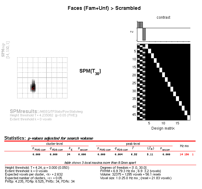
Save batch and review
Once you had added all the contrasts you want, you can save this batch
file (it should look like the batch_stats_rmANOVA_job.m file in the
SPM12batch FTP directory). Then run it, and when it has finished,
press “Results” from the SPM Menu window. Select the SPM.mat file in
the MEEG/TFStats/eeg directory, and from the new Contrast Manager
window, select the pre-specified T-contrast “Faces (Fam+Unf) \(>\)
Scrambled”. Within the Interactive window, when given the option, select
the following: Apply Masking: None, P value adjustment to control: FWE,
keep the threshold at 0.05, extent threshold voxels: 0; Data Type:
Time-frequency. The Graphics window should then show what is in Figure
10 below. Note the increase in power at 14Hz, 150ms that survives
correction (in all sensor types in fact). (If you examine the reverse
contrast of greater power for scrambled than intact faces, you will see
a decrease in the beta range, 22Hz, 475ms).