DCM for Evoked Responses
This chapter demonstrates an example of Dynamic Causal Modelling for Evoked Responses, based on the analyses as detailed by Tyrer, et al. (Tyrer et al., 2020). The purpose of the following analyses is to estimate the effective connectivity between sources of activity in the brain, in the context of a visual repetition memory paradigm.
In this chapter, the example here uses pre-existing data from a DCM for EEG study in Alzheimer’s disease patients and healthy aged controls (Tyrer et al., 2020). The key aims of this study were to investigate how inter-regional connectivity and within-region dynamics during implicit and explicit memory processing are implicated in Alzheimer’s disease, and to examine whether such connections in the right hemisphere provided compensation during these memory tasks. We hypothesized that hierarchical left-hemisphere specific connections may be weakened in the Alzheimer’s patient cohort compared with healthy aged controls.
One of the paradigms used in this study was a visual recognition task. Participants completed an encoding phase in which they were shown 100 images of nameable objects and were asked to press a button as they covertly named the object in the image. They then underwent EEG recording and during EEG recording they were presented with 100 images again, but 50 images were novel images, and 50 images were repeated from the encoding phase. These were presented in a random order, and participants had to register with a button press either whether or not they thought they had seen the image before. Therefore, this task consists of two different conditions: the novel image condition and the repeated image condition. The single-participant data used here is that of a healthy aged control participant in this visual recognition task.
Note
DCM is a hypothesis-driven method, and can be used to test specific hypotheses about the activity between sources in a network rather than simply being limited to asking questions about the strengths of the sources individually. DCM estimates effective connectivity as opposed to structural or functional connectivity, which is context-dependent. Rather than asking questions such as "How does one source increase the activity in another source?", with DCM you can ask context-dependent questions such as "How does one source have an influence over another source in a particular condition within a task?". DCM estimates this effective connectivity both within and between sources of activity, and these connections are examined in the context of regional activity changes, and also in a task-dependent fashion, so you can derive the way in which any experimental conditions that forms part of a task recruit or modulate any specific connections.
A further characteristic of DCM is that, through inversion of the model according to a Variational Bayesian scheme, this yields an approximation to the log-model evidence, which one can use to compare alternative models of the same data and make statistical inferences about which model best represents the data, i.e. has the highest model evidence.
Data
For this example we will use the pre-processed (band-pass filtered, epoched, artefact-corrected) EEG dataset1 saved in the files:
mfaeffspmeeg_examplecontrolsubject.mat
mfaeffspmeeg_examplecontrolsubject.dat
Three-dimensional source reconstruction and coregistration are also necessary for DCM for ERPs, so these steps should be performed in advance of DCM model specification.
Starting SPM for EEG
First, ensure that the main SPM directory is in your MATLAB path. Start
SPM 12 and select the M/EEG button, or type spm eeg in the command
line. This opens the SPM graphical user interface (GUI).
Constructing Your DCM
Once you have opened the SPM-GUI, you will see that the window is split into four main sections (from top to bottom): ‘Temporal pre-processing’, ‘Spatio-temporal modelling’, ‘Model specification, review and estimation’, and ‘Inference’. The button which opens the DCM GUI can be found on the right side of the ‘Spatio-temporal modelling’ section, which is second from the top in the SPM window. This opens a new graphics window, containing all the options required for you to specify your DCM (Figure 1.1).
The DCM GUI consists of five sections: section one allows you to load and save existing DCM files, and also select which type of model you want to apply; section two, ‘Data and Design’, is for selecting your data; section three, ‘Electromagnetic Model’, allows the specification of the spatial forward model; section four, ‘Neuronal Model’, is for specifying the connections within your model and inverting your DCM, and the final section contains additional buttons for viewing your results and conducting Bayesian Model Selection (BMS), which we will cover later.
Before the model can be specified, you must first select the data you wish to use for the model and progress through the sections in the fixed order laid out in the GUI, due to dependencies across each section, i.e. data selection > electromagnetic model > neuronal model. You can move both forward and backward through the sections by clicking the forward (>) and backward (\<) arrows respectively, and options within each section can be specified in any order.
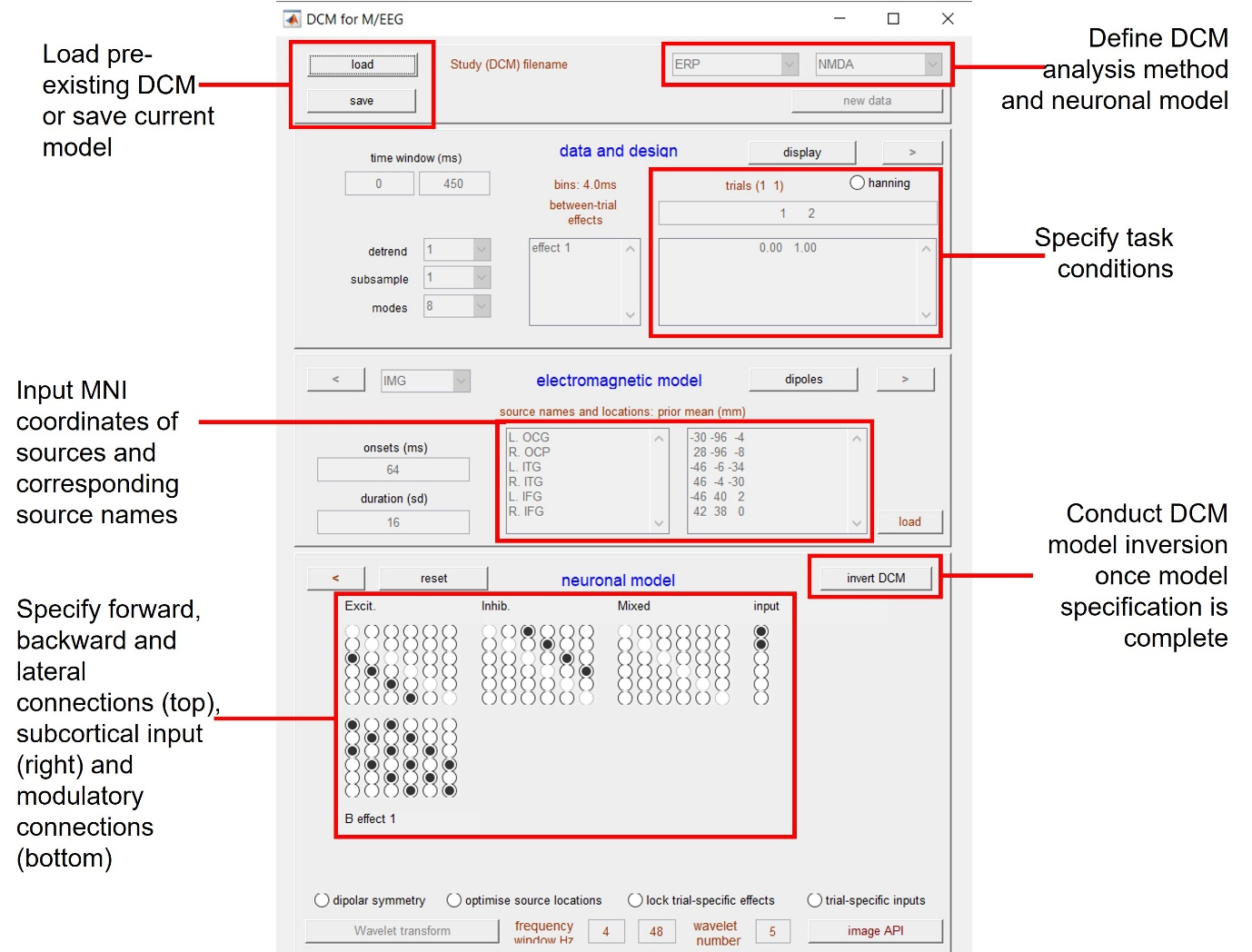
Load, Save and Model Selection
Starting with the first section in the DCM window, you can load a pre-existing DCM into the GUI by clicking ‘load’, or save a DCM you are currently working on by clicking ‘save’. You can save and load your DCM at any point during this specification process.
On the right side of this first section are two drop-down menus: the leftmost menu defines the type of DCM analysis that you wish to conduct. The default option is event-related potentials (ERP), i.e. DCM for evoked responses, Alternatively you could select DCM for induced responses (IND), cross-spectral density (CSD), neural field model (NFM), time-frequency model (TFM), or phase coupled responses (PHA). For this example we want to conduct DCM for evoked responses, so select the default option: ERP.
The rightmost drop-down menu allows you to select the type of neuronal model you wish to use. The default is once again ERP; other options are sensory evoked potential (SEP), canonical microcircuit (CMC), local field potential (LFP), neural mass model (NMM), mean field model (MFM), canonical microcircuit model (CMM), NMDA, CMM including an NMDA receptor model (CMM_NMDA), and neural field model (NFM). For this example, select NMDA. This neuronal model consists of a conductance-based neural mass model with three cell subpopulations, and includes a model of the NMDA receptor (Moran et al., 2011). The cell subpopulations consist of pyramidal cells (extra-granular cortical layers), inhibitory interneurons (extra-granular layers), and spiny stellate cells (granular layers).
Beneath these drop-down menus, click the button ‘new data’ to load your data and select the data file mfaeffspmeeg_examplecontrolsubject.mat. Data files will generally contain epoched data with multiple trials per condition. All data must be in SPM format to be used in DCM inversion.
Data and Design
In the next section below, ‘Data and Design’, you can define the peristimulus time window that the DCM will cover. In this example, by entering 0 in the left box and 450 in the right box, we select the time window 0-450 ms relative to the stimulus onset.
You can then specify the between-trial effects. In this task there are two conditions: novel images and repeated images. The text box on the right allows you to enter the trial indices of evoked responses in the data file you have selected. For the two conditions in this task, enter 1 and 2 in the box, corresponding to ‘novel’ and ‘repeated’ trials, respectively. To see which index is assigned to which trial condition, type into the command line:
This will display the list of condition labels and their associated indices. SPM should therefore display the following:
indicating that index 1 corresponds to the presentation of novel images and index 2 corresponds to the presentation of repeated images. The default name of ‘effect 1’ will be assigned to this effect by clicking somewhere outside the text box, and will appear in the larger leftmost text box.
The ‘detrend’ option allows you to remove any low-frequency drifts at the sensor level. Use this option to select the number of discrete cosine transform terms you would like to remove. However, if you do not wish to apply this, select the default value of 1 to simply remove the mean. Similarly, the ‘subsample’ option defines the factor used to down-sample the time bins. Here, this option can be left as the default value of 1. The third option, ‘modes’, allows you to define how many frequency modes to model in your data. The modes essentially describe the principal components of the data in sensor space. Generally, most of the physiologically relevant activity is encompassed by the first few modes, and the remaining modes just contain noise. The fewer modes you use, the quicker the DCM model inversion will be. Therefore, you might wish to run a DCM with a relatively large number of modes, and then see how many of the later modes contain relevant/important activity and how many contain noise. You might then run the model inversion again with a reduced, optimised number of modes. The default number of modes is 8, and for this example you can leave the number of modes as 8.
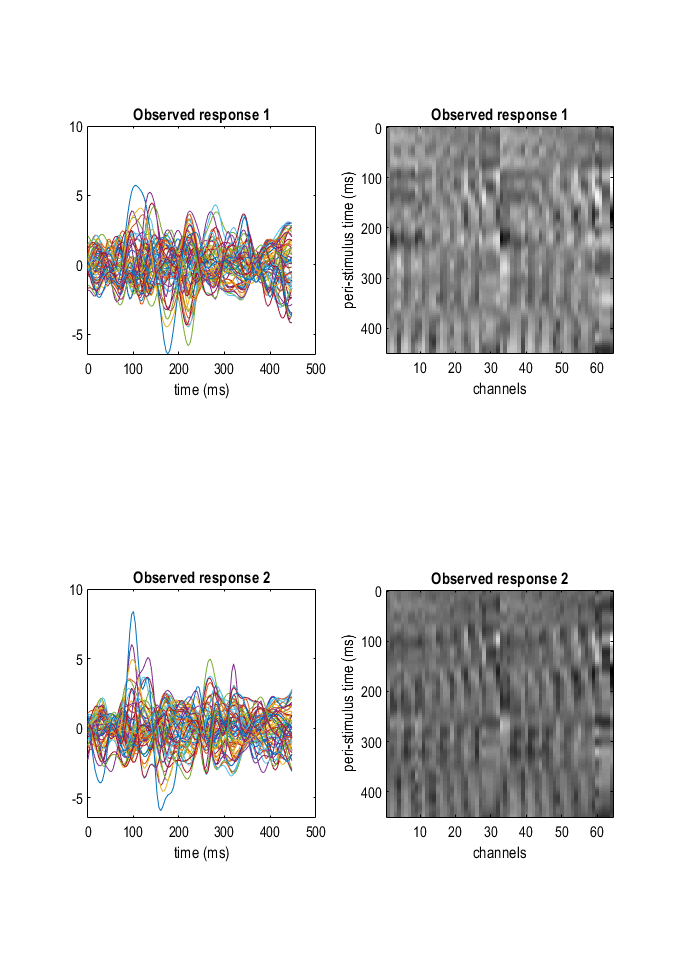
By clicking the ‘Display’ button on the top right, you can visualise the different observed responses for the novel condition (top row) and for the repeated condition (bottom row) in a separate graphics window (Figure 1.2). This displays the evoked responses for the two conditions you specified: each line in the left-hand plots represents the activity of a single channel. Visualising the data in this way is useful for determining your choice of time window and your selected detrending/subsampling options. You can change these options and click ‘Display’ again to see how changing these options affect the plots. To move onto the next section in the GUI, click on the forward arrow (>) on the right and this allows you to specify the electromagnetic model.
Electromagnetic Model
In this section, you can specify the spatial model of the evoked responses. With DCM for ERPs, there are four different options for how to ‘spatially model’ these evoked responses. This includes using a single equivalent current dipole (ECD) for each source; applying a patch on the cortical surface (IMG); or not using a spatial model and instead treating each individual channel as a source (LFP). For this example, select IMG.
By selecting IMG, you must then specify the prior source locations in MNI space (i.e. in mm in MNI coordinates). This would also be the case for DCMs using ECD. To specify source locations, you must enter a list of source names in the large box on the left, and the corresponding MNI coordinates in the large box on the right.
In the left large text box, enter:
L. OCG
R. OCP
L. ITG
R. ITG
L. IFG
R. IFG
In the right large text box, enter:
-30 -96 -4
28 -96 -8
-46 -6 -34
46 -4 -30
-46 40 2
42 38 0
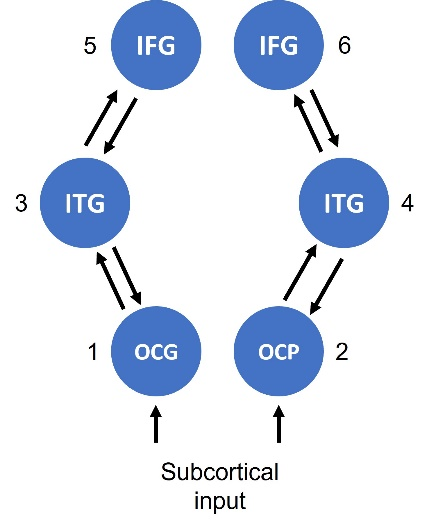
These sources correspond to the left Occipital Gyrus, right Occipital Pole, left Inferior Temporal Gyrus, right Inferior Temporal Gyrus, left Inferior Frontal Gyrus and right Inferior Frontal Gyrus respectively. Please see (Tyrer et al., 2020) for more details and information regarding source selection.
Alternatively, you can load a separate .mat file which contains the MNI coordinates of the sources you wish to specify. By clicking the ‘load’ button on the bottom right of the section, you can select the .mat file containing the MNI coordinates and SPM will auto-fill the right text box with the MNI coordinates. It is important to check that the MNI coordinates are in the correct order corresponding to the source names.
On the left side of the window, there are two additional options: ‘onsets (ms)’ and ‘duration (sd)’. The onset parameter determines when the stimulus, presented at 0 ms peristimulus time, is assumed to activate the cortical area to which it is connected. In DCM, you usually start modelling at the first large deflection in the data, which generally occurs at ~ 100 ms, therefore the default onset parameter is 64 ms to capture this first large deflection. For this example dataset, you can keep this as the default value. The duration parameter can be used to vary the width of the input volley for each of the inputs, if you wish to model the inputs more closely in the input structure. This can also be left at the default value of 16.
At the top of this section, there is a button labelled ‘dipoles’. Click this button, and the graphics window will display the relative locations of the sources that you’ve just defined in MNI space. The top half of the graphics window displays the coronal, sagittal and axial planes of the brain with the relative location of your first source highlighted by a yellow circle. You can switch which source is highlighted by using the drop-down menu in the lower right section of the window, labelled ‘Select dipole #‘. To visualise all relative source locations simultaneously, select ‘all’ in the drop-down menu. When viewing all source locations, each source is indicated by a different yellow shape. You can also drag the cross-hair around to visualise the locations of each source in 3D space.
In the main DCM GUI, click the forward (>) arrow once again to move onto the next section, in which you can define the neuronal model.
Neuronal Model
In this section, there are five matrices which enable you to define the connectivity within your model. The first four matrices (on the top row) enable you to define the connectivity structure of the model, and the last matrix (on the bottom row) specifies the modulatory connections, i.e. which connections are modulated by task-associated/experimental effects.
Connections are specified by indicating a source area, the area from which the connection originates, and the target area, the area which receives the incoming connection. In these matrices, the columns represent the sources that the connections are originating from, and the rows represent the regions that those connections are projecting to. For example, by selecting the radio button at (3,1), you are specifying a connection originating from source 1 and projecting to source 3, here, a connection from the left Occipital Gyrus to the left Inferior Temporal Gyrus.
The first three matrices, from left to right, define the forward, backward and lateral connections respectively; also known as the A matrices. In the NMDA model used here, forward connections project from pyramidal cells in the source area onto spiny stellate cells in the target area. Backward connections project from pyramidal cells in the source area to both inhibitory interneurons and pyramidal cells in the target area. Lateral connections project from pyramidal cells in the source area to all cell subpopulations in the target area.
The right-most matrix is the input matrix, or C matrix, which, in this example where we have a single input, takes the form of a 1xN vector, where N equals the number of sources we defined above in the electromagnetic model. This vector specifies which sources are receiving subcortical sensory input in the model.
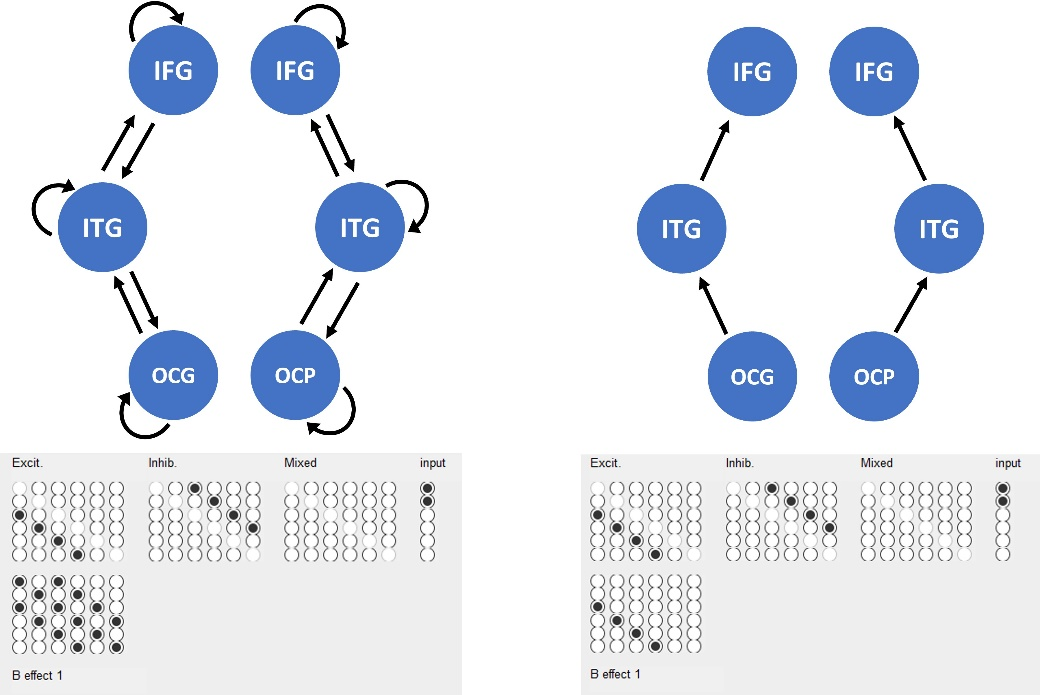
The final matrix (B effect matrix), on the second row, defines task-dependent modulatory connections. For this example, this defines the difference between novel and repeated image trials on specified connections. If you leave this matrix empty, the same model will be applied to all trials across all task conditions. Since we have one experimental condition, novel versus repeated images, there is only one B effect matrix.
For this example, define forward connections from L. OCG to L. ITG (3,1), L. ITG to L. IFG (5,3), R. OCP to R. ITG (4,2), and R. ITG to R. IFG (6,4). Define backward connections from L. ITG to L. OCG (1,3), L. IFG to L. ITG (3,5), R. ITG to R. OCP (2,4), and R. IFG to R. ITG (4,6). Here, we do not specify any lateral connections for this dataset. In the input vector, add subcortical input for L. OCG and R. OCP. In the B effect matrix, specify modulatory connections on the same forward and backward connections defined above, with the addition of self-connections on all sources. See Figures 1.3 and 1.4 for the connectivity map and buttons selected in the GUI for this model.
At the bottom of this section there are some additional options for the model. The first option is ‘dipolar symmetry constraints’; these can be used as a prior on the model if you want to model bilateral sources. This imposes a symmetry prior, and you can then run a model comparison between models either with or without this dipolar symmetry prior selected and examine the model fits between these two options. The second option, ‘optimise source locations’, allows you to relax zero variance priors on your specified source locations. The third option, ‘lock trial-specific effects’, enables you to enforce all trial-specific coupling gains to be the same, and the final option, ‘trial-specific inputs’, imposes trial-specific C parameter estimation.
Estimation and Results
Once you have completed the specification of your model, click ‘Invert’. Starting the DCM model inversion opens a second graphics window. At the top of the window you can see the hidden states of the two conditions: on the left hand side is the first condition, the novel image condition, and on the right hand side is the second condition, the repeated image condition.
In this plot there is one line for each cell subpopulation for each source in the model that we’ve specified, and this displays the hidden source dynamics within the model. In the centre panel, the predicted and observed responses are displayed in the principal component space or the mode space. Here, the dotted lines represent the real observed data and the solid lines represent the predicted response, and this is displayed for each of the 8 modes that were defined in the model.
At the bottom of the window are the conditional model parameters: on the left the conditional model parameters of the hidden states are shown, and on the right the conditional model parameters of the forward model (or observation model) are plotted.
During estimation, the main MATLAB command window shows the number of expectation-maximisation iterations that the model runs through throughout the inversion. It also displays the predicted change and actual change of free energy (F) following each iteration step. Once the model has fully estimated, SPM saves the results of the inversion in a DCM file, named DCM_*.mat, where * indicates the name of the original EEG data file specified for the model. At the bottom left of the DCM window there is a drop-down menu, which contains different options through which to view your results.
ERP (modes)
By selecting ‘ERP modes’, you can see the eight different modes, i.e. the essential principal components that are represented in the data. In these plots, dotted lines represent the observed data, and solid lines represent the model predictions, with different line colours indicating the different task conditions. In this example, most of the data has been captured within the first six or seven modes, so as an exercise, one could define and invert a similar model for the same data using fewer modes.
ERP (sources)
There is also the option to look at ERPs in source space. By selecting this option, the graphics window shows one plot for each of the six different sources as defined in our model. Each plot contains three different dash patterns of lines representing the three different cell subpopulations: population number one being the excitatory spiny stellates, population two being inhibitory interneurons, and population three are excitatory pyramidal cells. As above, different coloured lines are used to indicate the different task conditions.
Coupling (A)
To look at the estimated values for the coupling between sources, click ‘Coupling (A)’. This shows the conditional means of the estimates of the coupling strengths as defined in our A matrices – the matrices in which we defined the forward, backward and lateral connections within the model. This also shows the posterior probabilities, i.e. how likely these estimates are given the observed data.
Coupling (B)
Similar to the above, by clicking ‘Coupling (B)’ you can observe the estimated values and posterior probabilities for between-source coupling with the effect of task modulation, as defined earlier when setting up the B effect matrix(es) for the model.
Coupling (C)
Similar to ‘Coupling (A)’ and ‘Coupling (B)’, but in this case you can view the estimated values and posterior probabilities for inputs into the sources specified in the input vector to receive subcortical input.
Trial-specific Effects
This option displays bar plots representing the estimated connection strengths (%) and direction of modulating effects for each connection specified in the neuronal model, for each trial condition.
Input
By clicking ‘Input’, you can see the estimated input function: this is a gamma function with the addition of low-frequency terms.
Response, and Response (image)
The ‘Response’ option plots the data selected by the spatial modes defined in the model, back-projected into sensor space. Here you can view the (adjusted) observed data and the model predictions for each of the task conditions.
In the Response (image) option, you can see the same as with ‘Response’, but represented as a grey-scale image.
Scalp Maps
This displays the EEG scalp maps at different intervals across the time window as specified in the ‘Data and Design’ part of the model specification. Scalp maps are displayed for each task condition, for both observed data and model predictions.
Dipoles
By clicking ‘Dipoles’, you can view the locations of each source specified in the ‘Electromagnetic Model’ section of model specification. This option is only useful if you have selected ECD for the spatial model, therefore this option is not available for this example using IMG.
Bayesian Model Comparison
Now that you have successfully inverted your DCM, you can compare this with an alternative model of the same data. You must ensure that the first DCM you created is saved under a different name to the default; click the ‘Save’ button to rename the DCM file to make sure you don’t overwrite the file with the alternative model. To create an alternative model for this example, return to the ‘Neuronal Model’ section in the DCM window and edit the B effect matrix so that modulatory connections are only present on the forward connections (1.4). To invert the new model, click ‘Estimated’, ensuring that you do not use the previous posterior or prior estimates. Once the alternative model has been inverted, you can conduct Bayesian Model Comparison.
Click the ‘BMS’ button at the bottom of the DCM window, and this will open the batch editor for Bayesian Model Selection. You can also access this by returning to the SPM GUI, and clicking ‘Batch’ at the bottom. This will open an empty batch editor window. Click ‘SPM’ at the top, then DCM > Bayesian Model Selection > Model Inference. First, click ‘Directory’ and specify the directory in which the BMS output file will be saved. Click ‘Data’, then ‘New Subject’, then ‘New Session’. Click ‘Models’, and then click ‘Specify’: you can now select the DCM files in the file explorer for the two models you wish to compare. It is important to remember the order in which you select the DCM files; if you are comparing models across multiple subjects, the DCM files should be selected in the same order for every subject and session. If you wish to compare models for multiple subjects, you would click ‘New Subject’ for as many subjects you are analysing and select the DCMs for that subject.
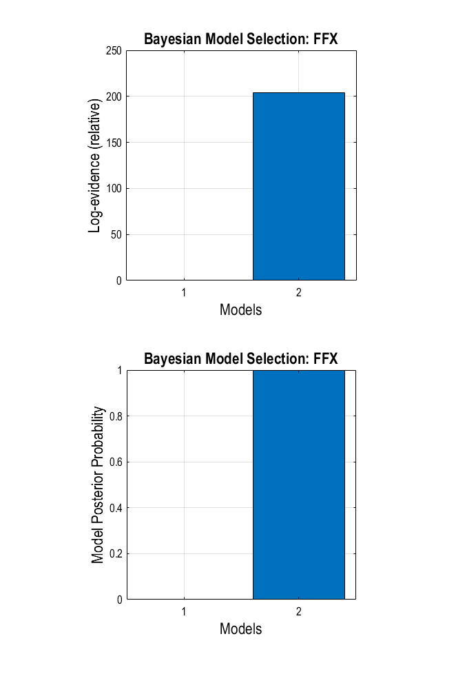
Select ‘Inference Method’ and click Fixed Effects (FFX), as in this example there are data and models for only one subject. Finally, click the green ‘Run’ arrow at the top to run the model comparison. The graphics window now displays two bar plots (1.5). The top plot shows the log-model evidence of the two models you have compared. The bottom plot shows the posterior probability for each model, given the data. A model is generally judged to be the best model for a given dataset compared with other models if its log-model evidence is greater than the log-model evidences of competing models by at least 3.
References
-
Moran RJ, Stephan KE, Dolan RJ, Friston KJ. Consistent spectral predictors for dynamic causal models of steady-state responses. Neuroimage 2011; 55: 1694-708.
-
Tyrer A, Gilbert JR, Adams S, Stiles AB, Bankole AO, Gilchrist ID, et al. Lateralized memory circuit dropout in alzheimer’s disease patients. Brain Communications 2020; 2: fcaa212.
-
DCM for ERP dataset: https://www.fil.ion.ucl.ac.uk/spm/data/dcm-erp/ ↩