DCM for Phase Coupling
This tutorial presents an extension of the Dynamic Causal Modelling (DCM) framework for analyzing phase-coupled data. A weakly coupled oscillator approach is employed to describe dynamic phase changes in a network of oscillators. The influence of one oscillator’s phase on another’s phase change is characterized using a Phase Interaction Function (PIF), as described in Penny et al. (2009). Although SPM supports PIFs specified with arbitrary order Fourier series, the interface is simplified by restricting users to simple sinusoidal PIFs when using the GUI.
Data
We will use the merged epoched MEG face-evoked dataset1, which is saved in the following files:
DCM-Phase requires a head model and coregistration. If you have been following the previous tutorials, these should already be available in the dataset. Otherwise, you should perform the ‘Prepare’ and ‘3D Source reconstruction’ steps described in the “Imaging source reconstruction” chapter. The latter includes the MRI, Co-register, Forward, and Save sub-steps.
Getting Started
To get started, follow these steps:
- Launch SPM and select “EEG” as the modality (located at the bottom-right of the SPM main window), or start SPM with the
spm eegcommand. Ensure that the main SPM directory is on your MATLAB path. - After calling
spm eeg, you will see SPM’s graphical user interface (GUI) in the top-left window. - Find the button for calling the DCM-GUI in the second partition from the top, on the right-hand side.
- Press the button to open the DCM-GUI (Figure dcm-ir:fig:1).
Data and Design
Follow these steps to set up the data and design for DCM-Phase:
- Switch the DCM model type to “PHASE”.
- Press “new data” and select the data file
cdbespm12_SPM_CTF_MEG_example_faces1_3D.mat. This file contains epoched data with multiple trials per condition. - On the right-hand side, enter the trial indices
1 2for the ‘face’ and ‘scrambled’ evoked responses. - In the box below the trial indices, specify experimental effects on connectivity by entering
1 0in the first row. This indicates that “face” trial types can have different connectivity parameters than “scrambled” trial types. - Click outside the box to assign a default name, “effect1”, to this effect. You can change this name to something more descriptive, such as “face”.
- Set the peristimulus time window to
1 300ms. - Select
1for “detrend” to remove the mean from each data record. - Optionally, use the
sub-trialsoption to select a subset of trials for analysis. For example, selecting2would analyze every second trial, and3would analyze every third trial. This can be helpful since DCM-Phase takes a long time to invert for all trials. In this example, we assume you used all trials (sub-trials set to 1). - Click the forward button (\(>\)) to proceed to the next stage, the electromagnetic model. You can press the red backward button (\(<\)) to return to the data and design part if needed.
Electromagnetic Model
DCM-Phase offers two options for extracting source data:
- ECD option: Use 3 orthogonal single equivalent current dipoles (ECD) for each source, invert the source model to get 3 source waveforms, and take the first principal component. This is suitable for multichannel EEG or MEG data.
- LFP option: Treat each channel as a source. This is appropriate for channels that already contain source data, either recorded directly with intracranial electrodes or extracted (e.g., using a beamformer).
In this example, we will use the ECD option and specify two source regions:
- In the left large text box, enter the source names:
- In the right large text box, enter the MNI coordinates for the sources:
Note that unlike DCM for evoked responses, DCM-Phase (like DCM-IR) does not optimize the parameters of the spatial model. It will project the data into source space using the spatial locations you provide.
After specifying the source names and coordinates, click the forward button (\(>\)) to proceed to the neuronal model. If you have not used the input dataset for 3D source reconstruction before, you may be asked to specify the parameters of the head model at this stage.
Neuronal Model
In this example, we will define a coupled oscillator model for investigating network synchronization of alpha activity:
- Enter the values
8and12to define the frequency window. The wavelet number is irrelevant for DCM-Phase.
After source reconstruction (using a pseudo-inverse approach), source data is bandpass filtered and the Hilbert transform is used to extract the instantaneous phase. The DCM-Phase model is then fitted using standard routines as described in (Penny et al. 2009).
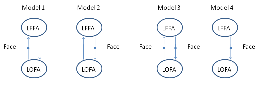
We will first fit Model 4, which proposes that alpha activity in region LOFA changes its phase to synchronize with activity in region LFFA. In this network, LFFA is the master and LOFA is the slave. The connection from LFFA to LOFA is allowed to be different for scrambled versus unscrambled faces.
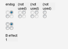
Configure the radio buttons as shown in Figure 1.2 and press the Invert DCM button. Estimating the model parameters may take up to an hour, depending on your computer’s speed.
Results
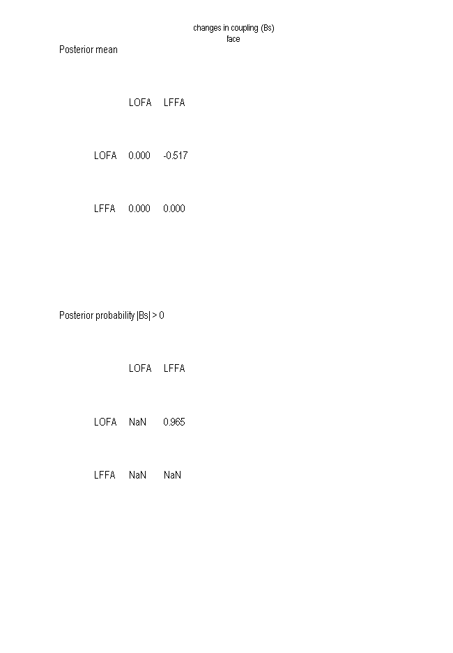
After estimation is finished, you can assess the results by choosing from the pull-down menu at the bottom (middle). The Sin(Data)-Region i option will show the sin of the phase data in region \(i\), for the first 16 trials. The blue line corresponds to the data, and the red line represents the DCM-Phase model fit. The Coupling(As) and Coupling(Bs) buttons display the estimated endogenous and modulatory activity shown in Figure 1.3.
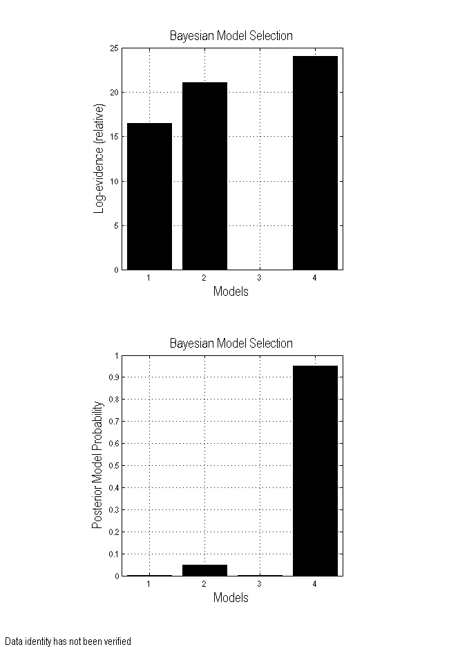
If you fit all four models shown in Figure 1.1, you can formally compare them using Bayesian Model Selection. To do this:
- Press the
BMSbutton. - Create a directory for the results (e.g.,
BMS-results). - For ‘Inference Method,’ select FFX (the RFX option is only viable if you have models from a group of subjects).
- Under ‘Data,’ select ‘New Subject,’ and under ‘Subject,’ select ‘New Session.’
- Then, under ‘Models,’ select the
DCM.matfiles you have created. - Press the green play button.
This process will produce the results plot shown in Figure 1.4. Based on these results, we can conclude that LFFA and LOFA act in a master-slave arrangement with LFFA as the master.
Extensions
In the DCM-Phase model accessible from the GUI, it is assumed that the phase interaction functions are of simple sinusoidal form, i.e., \(a_{ij} \sin(\phi_j - \phi_i)\). The coefficients \(a_{ij}\) are the values shown in the endogenous parameter matrices, for example, in Figure 1.3. These can then be changed by an amount \(b_{ij}\), as shown in the modulatory parameter matrices. It is also possible to specify and estimate DCM-Phase models using MATLAB scripts. In this case, it is possible to specify more generic phase interaction functions, such as arbitrary order Fourier series. Examples are given in Penny et al. (2009).
References
Penny, W. D., Litvak, V., Fuentemilla, L., Duzel, E., & Friston, K. J. (2009). Dynamic Causal Models for Phase Coupling. Journal of Neuroscience Methods, 183(1), 19–30.
-
Multimodal face-evoked dataset: http://www.fil.ion.ucl.ac.uk/spm/data/mmfaces/ ↩