Bayesian analysis
Specification
Press the Specify 1st-level button. This
will call up an fMRI specification job in the batch editor window. Then
-
Load the
categorical_spec.matjob file created for the classical analysis. -
Open
Subject/Session, highlightScans. -
Deselect the smoothed functional images using the
unselect alloption available from a right mouse click in the SPM file selector (bottom window). -
Select the unsmoothed functional images using the
^wa.*filter andselect alloption available from a right mouse click in the SPM file selector (top right window). The Bayesian analysis uses a spatial prior where the spatial regularity in the signal is estimated from the data. It is therefore not necessary to create smoothed images if you are only going to do a Bayesian analysis. -
Press
Done. -
Highlight
Directoryand select theDIR/bayesianfolder (directory) you created earlier (you will first need to deselect theDIR/categoricalfolder). -
Save the job as
specify_bayesian.matand press theRunbutton.
Estimation
Press the Estimate button. This will call
up the specification of an fMRI estimation job in the batch editor
window. Then
-
Highlight the
Select SPM.matoption and then choose theSPM.matfile saved in theDIR/bayesiansubfolder -
Highlight
Methodand select theChoose Bayesian 1st-leveloption. -
Save the job as
estimate_bayesian.joband press theRunbutton.
SPM will write a number of files into the output folder, including
-
An
SPM.matfile. -
Images
Cbeta_k.niiwhere \(k\) indexes the \(k\)th estimated regression coefficient. These filenames are prefixed with a “C”’ indicating that these are the mean values of the “Conditional” or “Posterior” density. -
Images of error bars/standard deviations on the regression coefficients
SDbeta_k.nii. -
An image of the standard deviation of the error
Sess1_SDerror.nii. -
An image
mask.niiindicating which voxels were included in the analysis. -
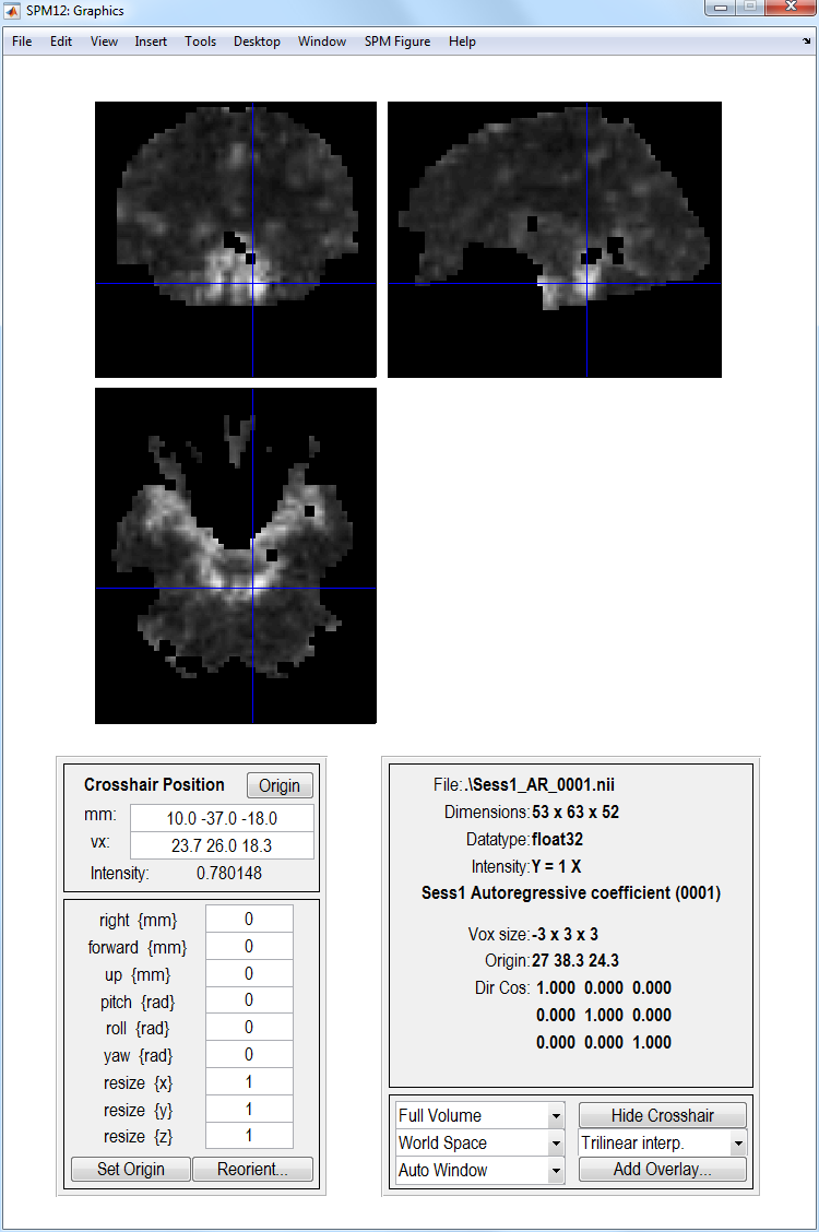
Images
Sess1_AR_p.niiwhere \(p\) indexes the \(p\)th AR coefficient. See eg. figure above. -
Images
con_i.niiandcon_sd_i.niiwhich are the mean and standard deviation of the \(i\)th pre-defined contrast.
Inference
After estimation, we can make a posterior inference using a PPM. Basically, we identify regions in which we have a high probability (level of confidence) that the response exceeds a particular size (eg, % signal change). This is quite different from the classical inferences above, where we look for low probabilities of the null hypothesis that the size of the response is zero.
To determine a particular response size (“size threshold”) in units of
PEAK % signal change, we first need to do a bit of calculation
concerning the scaling of the parameter estimates. The parameter
estimates themselves have arbitrary scaling, since they depend on the
scaling of the regressors. The scaling of the regressors in the present
examples depends on the scaling of the basis functions. To determine
this scaling, load the SPM.mat file and type in MATLAB
sf = max(SPM.xBF.bf(:,1))/SPM.xBF.dt (alternatively, press
Design:Explore:Session 1 and select any of the conditions, then read
off the peak height of the canonical HRF basis function (bottom left)).
Then, if you want a size threshold of 1% peak signal change, the value
you need to enter for the PPM threshold (ie the number in the units of
the parameter estimates) is 1/sf (which should be 4.75 in the present
case).1
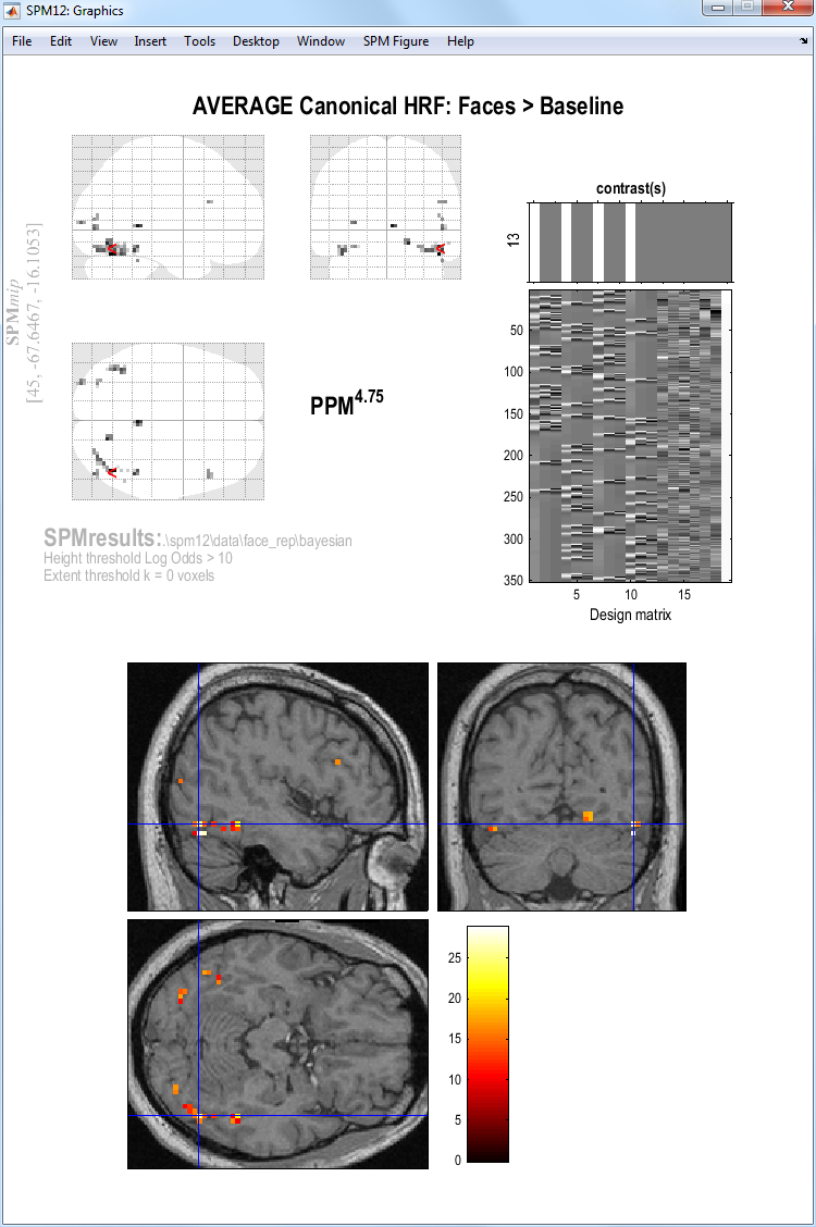
Finally, if we want to ask where is there a signal greater than 1% (with
a certain confidence) to faces versus baseline, we need to create a new
contrast that takes the AVERAGE of the parameter estimates for the
canonical HRF across the four conditions (N1 to F2), rather than the
default Positive effect of condition_1 contrast, which actually
calculates the SUM of the parameter estimates for the canonical HRF
across conditions (the average vs sum makes no difference for the
classical statistics).
-
Press
Results. -
Select the
SPM.matfile created in the last section. -
Press
Define new contrast, enter the nameAVERAGE Canonical HRF: Faces $>$ Baseline, press theT-contrastradio button, enter the contrast [1 0 0 1 0 0 1 0 0 1 0 0]/4, presssubmit,OKandDone. -
Apply masking ? [None/Contrast/Image]
- Specify
None.
- Specify
-
Effect size threshold for PPM
- Enter the value
-
Log Odds Threshold for PPM
- Enter the value
10.
- Enter the value
-
Extent threshold [0]
- Accept the default value.
SPM will then plot a map of effect sizes at voxels where it is 95% sure that the effect size is greater than 1% of the global mean. Then use overlays, sections, select the normalised structural image created earlier and move the cursor to the activation in the left hemisphere. This should create the plot below.
-
Strictly speaking, this is the peak height of the canonical component of the best fitting BOLD impulse response: the peak of the complete fit would need to take into account all three basis functions and their parameter estimates. ↩