DCM for Steady State Responses: Anaesthesia Depth in Rodent Data
Overview
This chapter describes the analysis of a 2-channel Local Field Potential (LFPs) data set using dynamic causal modelling. The LFPs were recorded from a single rodent using intracranial electrodes (Moran, Stephan, Jung, et al. 2009). We thank Marc Tittgemeyer for providing us with this data. The theory behind DCM for steady state responses (DCM-SSR) is described in (Moran, Stephan, Seidenbecher, et al. 2009).
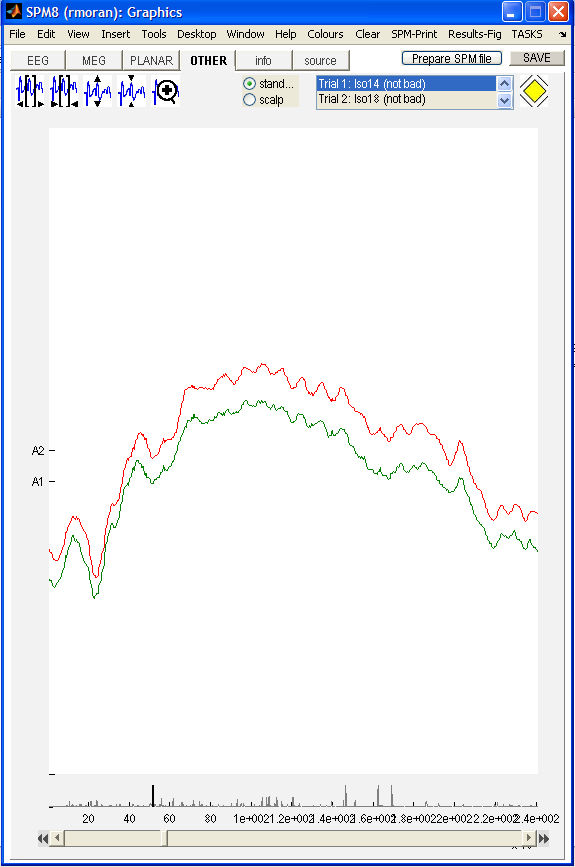
We measured local field potentials from primary (A1) and secondary auditory (A2) cortex in a rodent following the application of four different doses of the anaesthetic agent Isoflurane; 1.4, 1.8, 2.4 and 2.8mg. The rodent was presented with a white noise auditory input for several minutes at each anaesthetised level and time series recordings were obtained for the entire epoch. We performed a steady state DCM analysis using different models, defined according to the extrinsic connections between A1 and A2.
Using Bayesian model comparison we found very strong evidence (Bayes
Factor\(_{1,2}\) \(>\) 100) in favour of a model comprising a network of two
neural masses connected by forward (excitatory) and backward
(inhibitory + excitatory) connections (m1). This outperformed both a
model comprising two neural masses with forward (excitatory) connections
only (m2) and a model comprising two neural masses and lateral
(inhibitory + excitatory + excitatory) connections only (m3). Within
this best performing model we observed changes in forward and backward
connections dependent on dose. The strength of inhibitory backward
connections increased with successive anaesthetic dose, constituting a
greater GABAergic influence postsynaptically for higher doses.
Conversely, the solely excitatory forward connections reduced in
strength with successive doses
In what follows, these results will be recreated step-by-step using SPM8.
To proceed with the data analysis, first download the data set from the
SPM website1. The data comprises a data file called
dLFP_white_noise_r24_anaes.dat and its corresponding mat file
dLFP_white_noise_r24_anaes.mat. This has been converted from ASCII
data using spm_lfp_txt2mat_anaes.m also on the website and
subsequently downsampled to 125 Hz. The conversion script can be altered
to suit your own conditions/sampling parameters.
The data
-
To check data parameters after conversion using ASCII files: in the SPM M/EEG GUI press Display/M/EEG.
-
In our data set we can see there are five trials: four depths of anaesthetic:
Iso14,Iso18,Iso24andIso28and one awake trialawake. -
We can also see that the data are clean for both the A1 and A2 channels, to view this press other, as the data are LFP type.
-
We are now ready to begin the DCM analysis. To open the DCM GUI press DCM in the SPM M/EEG GUI.
LFP_white_noise_r24_anaes.mat one can check
the data quality, length, trials and sampling parameters. Dynamic Causal Modelling of Steady State Responses
-
Before you begin any DCM analysis you must decide on two things: the data feature from your time series and the model you wish to use.
-
For our long time series we will examine the steady state and so in the top panel of the DCM GUI select SSR in the data drop-down menu.
-
Next in the second drop down menu we select our model. For this LFP data we employ the LFP model and so this is then selected.
-
Then we are ready to load our data: press new data and select the file
dLFP_white_noise_r24_anaes.mat. -
Press the red arrow to move forward.
-
The second panel allows you to specify the data and design. We will use the first 30sec of the time series for our analysis. To specify this timing enter
1and30000in the time window. -
Next we select the detrending parameters which we set to
1for detrend,1for subsample (as the data has already been downsampled) and2for the modes (in this case this is the same as the number of channels) using the drop down menus. -
We can then specify which trials we want to use. Since we are interested in the anaesthetized trials we enter
1 2 3 4under the trials label andeffect1 effect2 effect3in the between trial effects panel. Next we specify the design matrix. This is entered numerically in the large panel. Since we have 4 trials and 3 between trial effects (one less) we enter a matrix with rows:[ 0 1 0 0 ] (row 1), [0 0 1 0] (row 2) and [0 0 0 1] (row 3). This will allow us to examine “main effect” differences between the four conditions.2 -
Press the red arrow to move forward.
-
The third panel contains the spec for the electromagnetic model. This is very simple for LFPs. In the drop down menu select LFP. In the source names panel, enter
A1andA2. You are finished. -
Press the red arrow to move forward.
-
At this point all that is left to specify is the neuronal model. We wish to compare three different models so we can save the specifications so far using the save button and reload the above specs for all three neuronal models.
-
To specify the neuronal model, load the DCM (that you just saved) as it has been so far specified.
-
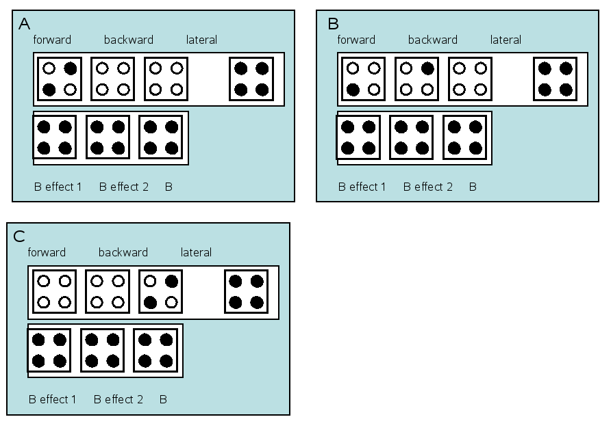
Our first model is the forward model. So we specify forward connections from A1 to A2 and forward connections from A2 to A1 (Fig 1.2)
-
We also specify the input. In our experiment we assume input at both sources.
-
We finally specify the B effects where we enter our hypothesis of connectivity changes between trial 1 (Iso1.4mg) trial 2 trial 3 and trial 4. Changes will be specified relative to trial 1.
-
We enter the off diagonal entries to correspond to forward connections (as entered in the above panel) and the main diagonal entries to specify intrinsic connectivity changes with A1 and A2 due to (anaesthetic) condition.
-
Finally we enter the frequencies we are interested in: we will fit frequencies from 4 to 48 Hz.
-
To invert the model press invert DCM.
-
Repeat the procedure after loading the saved specs and repeating for new neuronal models as per Fig 1.2.
Results
-
Once all models have run, we compare their evidences to find to best or winning model.
-
To do this press the BMS button. This will open the SPM batch tool for model selection. Specify a directory to write the output file to. For the Inference method select
Fixed effects(see (Stephan et al. 2009) for additional explanations). Then click on Data and in the box below click on New: Subject. Click on Subject and in the box below on New: Session. Click on models and in the selection window that comes up select the DCM mat files for all the models (remember the order in which you select the files as this is necessary for interpreting the results). Then run the model comparison by pressing the green Run button. You will see, at the top, a bar plot of the log-model evidences for all models [dcm-ir:fig:6]. At the bottom, you will see the probability, for each model, that it produced the data. By convention, a model can be said to be the best among a selection of other models, with strong evidence, if its log-model evidence exceeds all other log-model evidences by at least 3. You can also compare model evidences manually if you load the DCMs into Matlab’s workspace and find the evidence in the structure underDCM.F -
We can then examine the fits and posterior parameters of the winning model by loading it into the DCM GUI and selecting options from the drop down results menu.
-
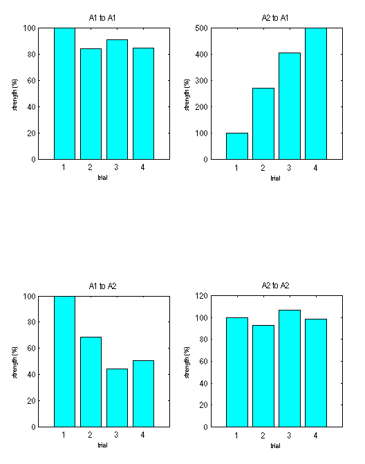
In the "trial specific effects" window we are interested particularly in the off-diagonal entries specifying trial specific extrinsic connectivities. Here for the f-b model we see increasing inhibitory (backward) connectivity and decreasing (forward) connectivity for increasing Isoflorane levels (Fig 1.3.
-
Anaesthesia Depth in Rodent Dataset: http://www.fil.ion.ucl.ac.uk/spm/data/dcm_ssr/ ↩
-
The effect of anaesthesia could also be specified as a single linear effect, for instance by using a vector of mean-corrected anaesthetic concentrations: [14 18 24 28] - mean([14 18 24 28]) = [-7 -3 3 7]. Here we specified 3 separate effects to show that even when the effects are specified separately, there is a consistent trend in connectivity changes with the increase in anaesthetic concentration. ↩