MEG source localisation
Overview
In this section we will generate some simulated data to show how the inversion algorithms compare when the ground-truth is known.
Simulation
The easiest way to simulate M/EEG data is by replacing data from an
existing experimental recording in which sensor locations/head position
etc are already defined. You can do this using the batch editor. Start
the batch editor (Batch button) on main panel. Then from the dropdown
menu SPM: select M/EEG; select Source reconstruction; select
Simulation of sources on cortex. You will see the following menu:
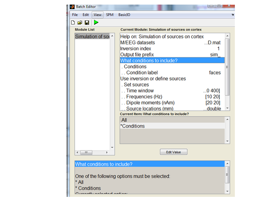
You can use any SPM file you like to provide the basic simulation set up: this file will include information on sensor locations, triggers, head model. As an example we can use the preprocessed multimodal face-evoked MEG dataset1. So for M/EEG dataset select
cdbespm12_SPM_CTF_MEG_example_faces1_3D.mat
Inversion index allows you to determine which forward model/ inversion
is used to simulate data, leave this at the default value (1) for now.
Output file prefix allows you to specify the prefix to be added to the
new file. Under ‘what conditions to include’, you can either specify to
simulate data in all experimental conditions ‘All’ or in specific
conditions only. Here we want to test between conditions so we will
simulate data in only one condition. Select the Conditions option and
for Condition labe’ type
faces
The next option Use inversion or define sources allows you to either
re-generate data based on a previous source reconstruction (and vary the
SNR) or to set up a number of active sources on the cortical surface. We
will use the last option, select Set sources. You can use the default
options for now which defines two sources at different frequencies in
approximately the auditory cortices.
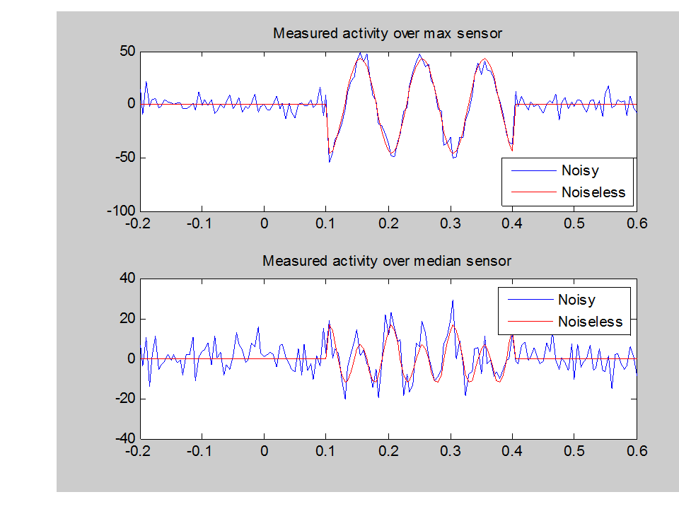
That is, the two dipoles are currently set to be on (at 10 and 20Hz) during the faces condition and off during the scrambled condition.
This file has dipoles at [52, -25, 9] and [-52, -25, 9] in MNI space. The dipoles are energized at 10Hz and 20Hz from 0.1 to 0.4 seconds (Figure 1.1). In each epoch the activation profile is identical, the channel data will be slightly different due to the white noise added. The green arrow in the top left menu bar should light up when all the essential parameters have been input and you can press it to run the simulation.
You can visualise the data trial by trial if you like by using the main menu Display/MEEG button.
Imaging solutions for evoked or induced responses
There are two pathways you can take to analyse the data. Either with the GUI buttons or with the batch interface.
Firstly lets use the GUI to check that the data is ready for source
inversion. On the main menu Click 3D Source Reconstruction. Press
Load. Select the new simulated data file
sim_cdbespm12_SPM_CTF_MEG_example_faces1_3D.mat.
Moving left to right along the bottom panel you will notice that all of the buttons (MRI, Co-register, Forward Model) are active. This means that the preprocessing stages have already been carried out on these data (see multi-modal evoked responses chapter).
The advantage of the batch interface is that you can then build up large and automated analysis pathways, it also is a little more flexible so it has more functionality.
So restart the Batch editor from the main menu Batch. Then from the
SPM drop-down menu select M/EEG / source reconstruction /
Source inversion.
Select the new simulated data file
sim_cdbespm12_SPM_CTF_MEG_example_faces1_3D.mat. Now we wish to invert
all conditions using the same assumptions (and then compare between
conditions afterwards) so under ‘what conditions to include’ select
‘All’. At this point we can now try out inversion algorithms with
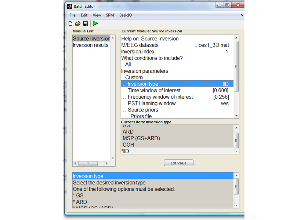
different implicit assumptions. Under Inversion parameters select
Custom. We will modify inversion type in the subsequent sections.
Select IID for minimum norm assumptions for now. For the
Time window of interest select from 0 to 600ms. For the
frequency window of interest select 0 to 80 Hz (our data were
simulated at 10 and 20Hz between 100 and 400ms). All the other settings
should remain as default.
IID (minimum norm)
We will start off with the traditional minimum norm solution: the ‘IID’
inversion type option . This starts by assuming that all source elements
contribute something to the measured data. The constraint is that the
total power (in the sources) should be minimised. Press Invert. Under
reconstruction method press Imaging. For All conditions or trials
press Yes. For model press Custom. Model inversion IID. Under
Time-window “0 600”. For PST Hanning select Yes. For High-pass (Hz)
select 1 for Low-pass (Hz) select 48. For Source priors, select
No. Under Restrict solutions select No.
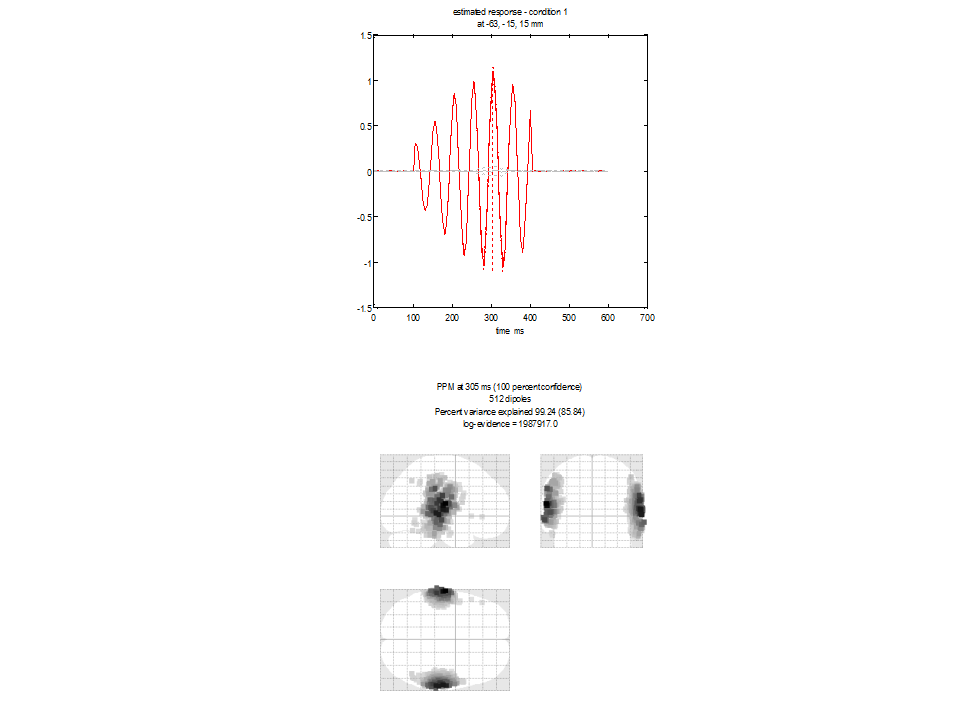
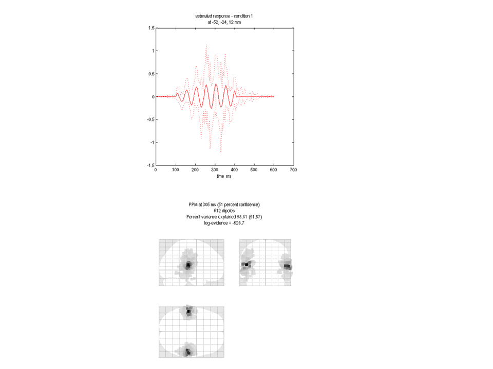
We see the anticipated minimum norm result. The current density estimate is diffuse and relatively superficial due to the minimum energy constraint. Note the log-evidence 1987917 (this value depends on the data - so value of the log evidence you see may be different but it is this value relative to those following which is important). The top panel shows two time-series extracted from the mesh vertex (location given at the top of the panel) with highest posterior probability. The red line corresponds to the first condition (faces). Note the sinusuoidal time-series which should correspond in frequency to the source simulated on that side of the brain. The grey line corresponds to the other condition (scrambled) in which no data were simulated.
Smooth priors (COH)
The COH, under Inversion type, option allows the mixture of two
possible source covariance matrices: the minimum norm prior above and a
much smoother source covariance matrix in which adjacent sources are
correlated (over the scale of a few mm). Select COH as the custom
source reconstruction and run the batch again.
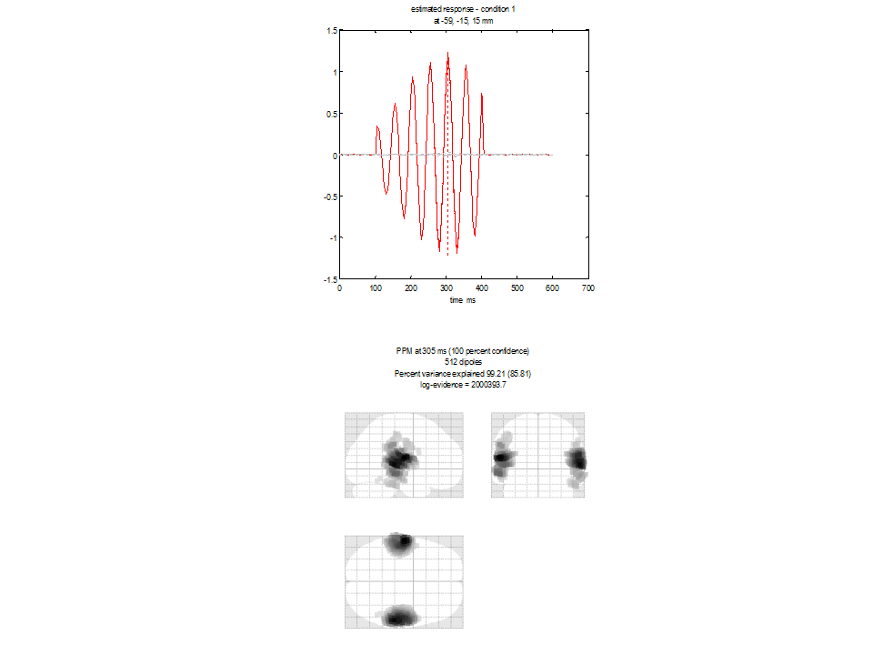
You will see a plot similar to Figure 1.5 appear. The lower panel shows the glass brain in which bilateral sources are apparent. The upper panel shows the time-series of the source with the largest amplitude. In this case the peak activation is identified at location 59,-15, 15mm. The 20Hz time-course (associated with this source) is also clearly visible in the top panel. Log evidence is 2000393 (again this number may be different in your spm version). Note both that the source reconstruction is more compact and that the log evidence has increased over the IID solution.
The Multiple sparse priors algorithm
In contrast to IID or COH, the greedy search routine used in MSP builds
up successive combinations of source configurations until the model
evidence can no longer be improved. Select GS as the inversion type
and run the batch again. You will see a plot similar to
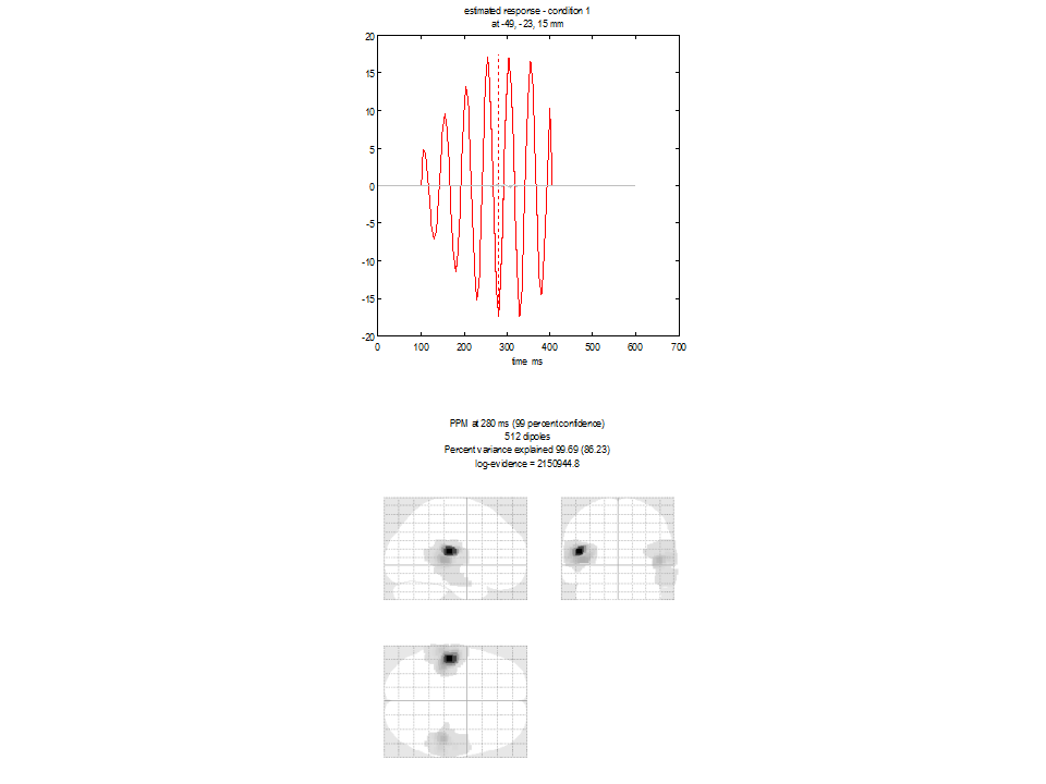
Figure 1.6 appear. The lower panel shows
the glass brain in which bilateral sources are apparent. The upper panel
shows the time-series of the source with the largest amplitude. Again
the source reconstruction is compact with log evidence is 2150944. Note
both that the source reconstruction is more compact and that the log
evidence has increased over the IID and COH solutions. There are two
more options in the basic MSP implementation- ARD- based on the removal
of patches that contribute little to the model evidence; and the use of
both schemes ‘ARD and GS’ in which both methods provide candidate source
covariance estimates which are then combined. You can try out these
other options for yourself and note the model evidences (which will be
directly comparable as long as the data do not change).
Making summary images
Often we will interested in some summary of conditions over a specific time-frequency window. We can add in an extra module to the batch script to produce such an output. .
From the SPM drop down menu click M/EEG/ Source reconstruction/
Inversion results. Now for M/EEG dataset, click Dependency- and
press OK to link the output of the previous function (the inversion) to
the input of this one. We can now produce power images per condition
based on a 0 to 600ms time window and a 0 to 80Hz frequency window. For
Contrast type select Evoked and for output space and format select
MNI and Mesh .
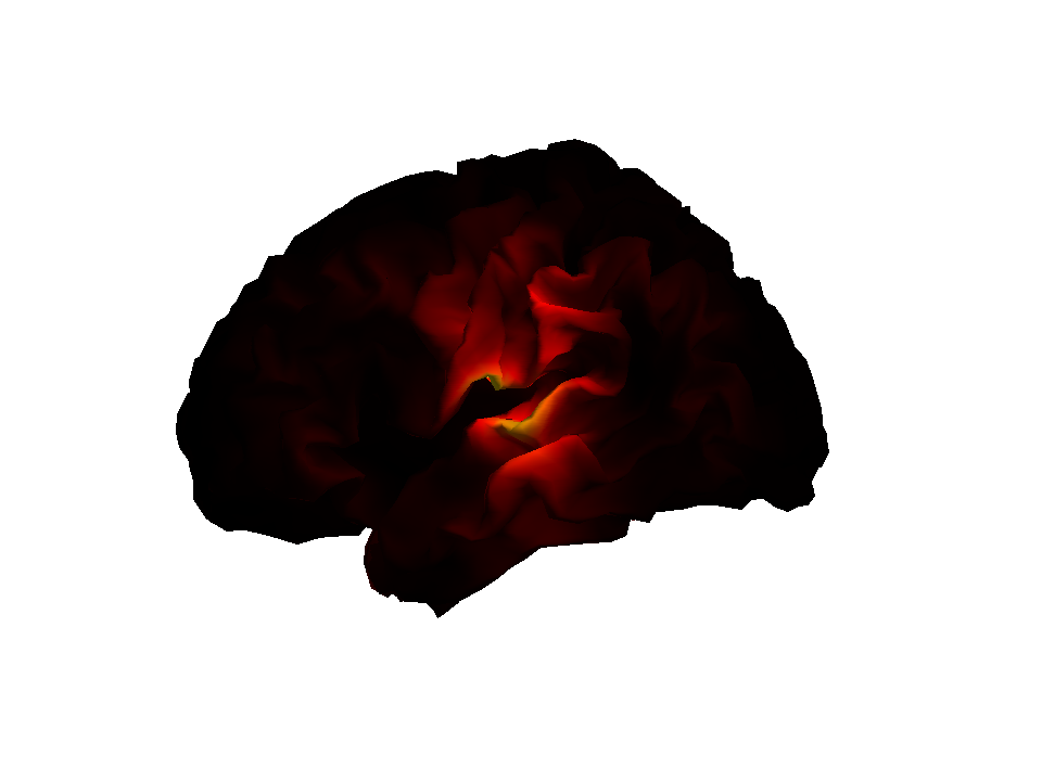
You should now be able to run the complete batch which re-does the
inversion and outputs two surface meshes (one for each condition). You
can view these meshes from the main menu : Render/ Display. The
output image for the face condition (and the IID algorithm) is shown
below.
Other MSP options
The MSP algorithm is optimized to give the simplest source distribution
that explains the most data. However the library of priors (possible
patch locations) must be pre-specified in advance. This could
potentially cause a problem if the source of interest were not precisely
centred on one of the patches in the default library. To this end Jose
David Lopez (Conf Proc IEEE Eng Med Biol Soc. 2012;2012:1534-7.) has
produced a version of MSP which uses multiple random patch libraries to
invert the same data several times. We can make a new batch file for
this. So restart the Batch editor from the main menu Batch. Then from
the SPM drop-down menu select M/EEG / source reconstruction /
Source inversion, iterative.
Select Classic as the custom source reconstruction algorithm- this is
basically the original version of the MSP algorithm without any
re-scaling factors to allow mixing of modalities or group imaging. It is
advantageous in many cases as the lack of these scaling factors means
that it is a true generative model of the data (and it becomes possible
to test between different head positions etc). Note however that these
differences in pre-processing mean that at the moment the data entering
the inversion (for custom and classic options) are different and so it
is not possible to compare between solutions from these two pipelines.
The rest of the parameters (time, frequency windows etc) can remain as
they were in the last section. The new options are the choice over the
number of patches in the library and the number of iterations. You can
play with these parameters to adjust the relative burden of computation
time. For example- allowing just 2 patches and many iterations will make
this something like a (cortically constrained) multiple dipole (patch)
fit. Alternatively, having lots of patches initially will mean the
computation time is spent on pruning this set (with ARD or GS etc). You
also have control over the number of temporal and spatial modes which
will be used here (this makes it easier to compare between models where
the lead field matrix has changed). The algorithm returns the current
distribution based on the patch set with maximum free energy.
An alternative to many spatial priors is to have a single prior that is
optimised using functional constraints. This idea was put forward by
Belardinelli P et al. PLoS One. 2012;7(12). Here a single candidate
source covariance is estimated using beamformer priors and then
regularized (in much the same way as IID and COH matrices are) in the
Bayesian framework. You can access this by selecting EBB (Empirical
Bayes Beamformer) as the inversion type; but you should set the number
of iterations here to 1 (as there is only a single prior and it will not
change over repetitions).
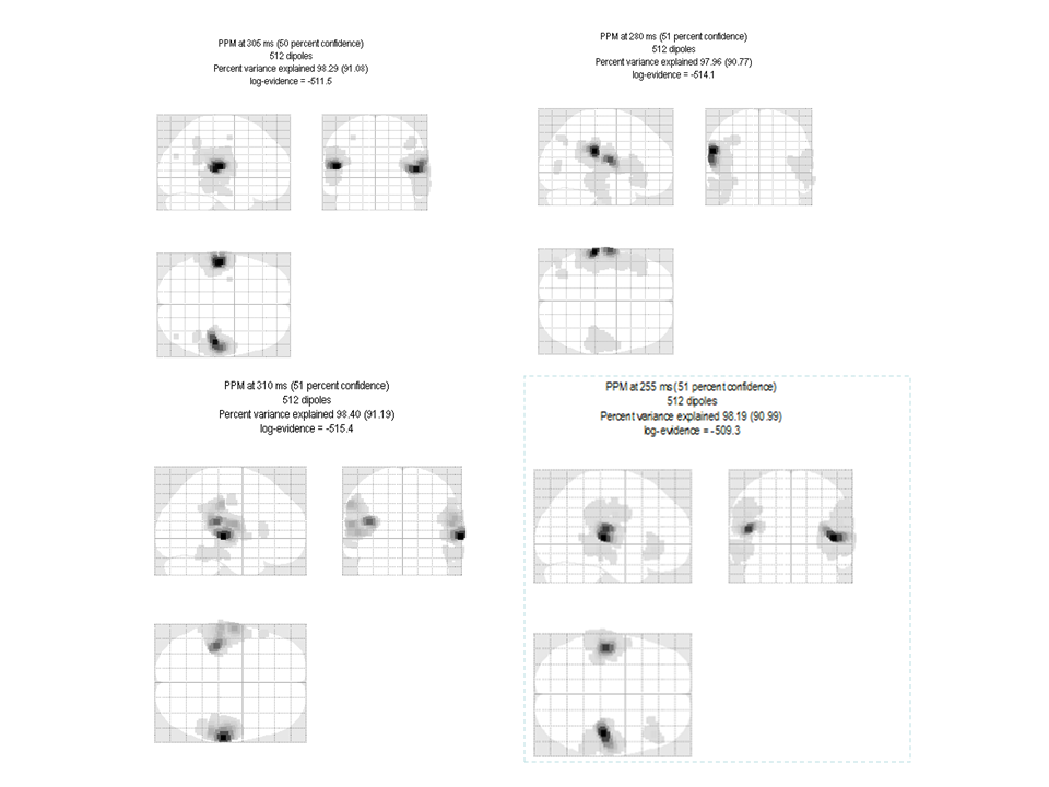
You can see that the beamformer image is much more focal than any other image type (and it is fast to compute). However there will be many situations in which it is sub-optimal (such as if you were to simulate two correlated sources). In Belardinelli et al. the authors found that this failure was reflected in the free energy; meaning that it is still possible to directly compare this solution with GS , IID etc.
Dipole fitting to the average
Up until this point the analysis we have used could have been applied to
either induced or evoked changes in electrical activity. The only
difference being that it would not have made much sense to look at the
MSPs for specific time-instants in the induced case and we would have
proceeded directly to look for changes in a time-frequency window. To
examine the dipole fit routine we will however concentrate on the
averaged data file which will contain only evoked changes. For this
final section we will revert back to the main gui. Press Average.
Select the simulated data file and leave all of the other options as
default.
Press 3D source Reconstruction.
Load/preview the data
In the main menu click on the drop-down Display menu. Select M/EEG.
For the dipole fitting we are going to use averaged MEG data, this is
prefixed with an “m” in SPM. You can generate this file by averaging the
epoched file that we have used until now. Select the file
msim_cdbespm12_SPM_CTF_MEG_example_faces1_3D.mat.
The two sources we simulated were at 10Hz an 20Hz frequency so we can select times when only one or both of them were active. At 235ms there is only one dominant source and at 205ms both sources are clearly visible at the sensor level.
We will now move on to explore Bayesian dipole fitting to these two time instants.
Inversion
In the main menu window, select 3D Source Reconstruction. Click Load
and select the averaged simulated dataset above. Proceed by pressing the
Invert button. Select the VB-ECD button.
Fitting a single dipole with no priors
At the time_bin or average_win prompt enter “235”. For
Trial type number choose “1” (we want to model the faces data). At the
Add dipoles to model click Single. For location prior click
Non-info. For Moment prior click Non-info. At the
Add dipoles to 1 or stop? prompt click stop. At the Data SNR (amp)
leave as default 5. Leave the default number of iterations at “10”.
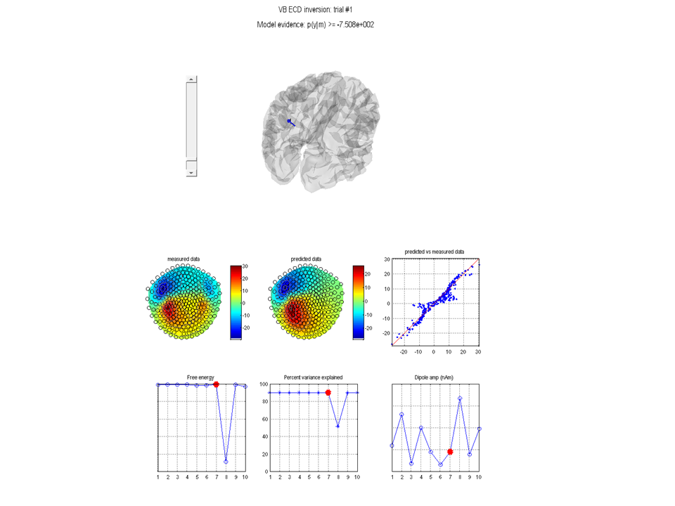
You will see the 10 successive fits of the same data using a random
starting location and moment. At each fit maps of the predicted and
simulated data along with free-energy values and percent variance
explained are shown. The final plot will be similar to
Figure 1.10 where the model (i.e. dipole)
which maximised the evidence (the best iteration is shown with a red
dot) is displayed. Note down the model evidence (in this case -7.508e2,
but the absolute value in your implementation may be different). The
Bayesian dipole fit algorithm will be most useful when one has some
prior knowledge of the sources (such as location, orientation or
symmetry). Typical dipole fit algorithms fit 3 location parameters per
dipole and then estimate the moment through a pseudo-inverse. The VB-ECD
algorithm however fits 6 parameters per dipole as the moments are also
allowed prior values. That is, if you have no prior knowledge then the
Bayesian method will be generally less robust than such fitting methods
(as more parameters are being fit). However it is when prior knowledge
is supplied that the Bayesian methods become optimal.
Fitting a single dipole with reasonable and unreasonable priors
We will now provide some prior knowledge to the dipole fit perhaps led
by the literature or a particular hypothesis. In this case we know the
answer, but let us specify a location a couple of cm from where we know
the source to be and try the fit again. At the time_bin or average_win
prompt enter “235”. For Trial type number choose “1” (we want to model
the faces data). At the Add dipoles to model click Single. For
location prior click Informative. For the location enter “-62 -20
10”. For prior location variance leave at “100 100 100” mm\(^2\). This
means that we are not sure about the source location to better than 10mm
in each dimension. For Moment prior click Non-info. At the
Add dipoles to 1 or stop? prompt click stop. Leave the default
number of iterations at “10”. Again you will get a final fit location
and model evidence (-7.455e2), which should have improved (be more
positive) on the evidence above (because in this case our prior was more
informative). Now go through exactly the same procedure as above but for
the prior location enter “-62 +20 10”, i.e. on the wrong side of the
head. You will note that the algorithm finds the correct location but
the evidence for this model (with the incorrect prior) is lower
(-7.476e2).
Fitting more dipoles
We will start by examining the time instant at which we can clearly see
a two-dipolar field pattern. At the time_bin or average_win prompt
enter “205” (not that we are now changing the data so the subsequent
evidence values will not be comparable with those at 235ms). For
Trial type number choose “1”. At the Add dipoles to model click
Single. For location prior click Informative. For the location
enter “62 -20 10”. For prior location variance enter “400 400 400”
mm\(^2\), that is, the prior standard deviation on the dipole location is
20mm in each direction. For Moment prior click Non-info. At the
Add dipoles to 1 or stop? prompt click Single. For location prior
click Informative. For the location enter “-62 -20 10”. For prior
location variance enter “400 400 400” mm\(^2\). At the
Add dipoles to 1 or stop? prompt click stop. Leave the default
number of iterations at “10”. Note down the final model evidence
(-2.548e2).
Alternatively we can exploit the fact that we have prior knowledge that
the dipoles will be approximately left-right symmetric in location and
orientation (this means we have fewer free parameters or a simpler
model). At the time_bin or average_win prompt enter “205”. For
Trial type number choose “1”. At the Add dipoles to model click
Symmetric Pair. For location prior click Informative. For the205
location enter 62 -20 10. For prior location variance enter “400 400
400” mm\(^2\). For Moment prior click Non-info. At the
Add dipoles to 2 or stop? prompt click stop. Leave the default
number of iterations at “10”. Note that the final locations are
approximately correct, but importantly the model evidence (-5.235e2) is
lower than previously. Given this information one would accept the (more
complex) two distinct dipole model over the symmetric pair model.
-
Multimodal face-evoked dataset: http://www.fil.ion.ucl.ac.uk/spm/data/mmfaces/ ↩