EEG analysis 
First change directory to the EEG subdirectory (either in MATLAB, or via the “CD” option in the SPM “Utils” menu).
Convert
Press the Convert button and select the
faces_run1.bdf file. At the prompt “Define settings?” select “just
read”. SPM will now read the original Biosemi format file and create an
SPM compatible data file, called spm8_faces_run1.mat and
spm8_faces_run1.dat in the current MATLAB directory. After the
conversion is complete the data file will be automatically opened in
SPM8 reviewing tool. By default you will see the “info” tab. At the top
of the window there is some basic information about the file. Below it
you will see several clickable tabs with additional information. The
“history” tab lists the processing steps that have been applied to the
file. At this stage there is only one such step - conversion. The
“channels” tab lists the channels in the file and their properties, the
“trial” tab lists the trials or in the case of a continuous file all the
triggers (events) that have been recorded. The “inv” tab is used for
reviewing the inverse solutions and is not relevant for the time being.
Note that the detailed information in the tabs will not be available for
MATLAB versions older than 7.4. At the top of the window there is
another set of tabs. If you click on the “EEG” tab you will see the raw
EEG traces. They all look unusually flat because the continuous data we
have just converted contains very low frequencies and baseline shifts.
Therefore, if we try to view all the channels together, this can only be
done with very low gain. If you press the “intensity rescaling” button
(with arrows pointing up and down) several times you will start seeing
EEG activity in a few channels but the other channels will not be
visible as they will go out of range. You can also use the controls at
the bottom of the window to scroll through the recording. If you press
the icon to the right of the mini-topography icon, with the rightwards
pointing arrow, the display will move to the next trigger, shown as a
vertical line through the display. (New triggers/events can be added by
the rightmost icon). At the bottom of the display is a plot of the
global field power across the session, with the black line indicating
the current timewindow displayed (the width of this timewindow can be
controlled by the two leftmost top icons).
Downsample
Here, we will downsample the data in time. This is useful when the data
were acquired like ours with a high sampling rate of 2048 Hz. This is an
unnecessarily high sampling rate for a simple evoked response analysis,
and we will now decrease the sampling rate to 200 Hz, thereby reducing
the file size by more than ten fold and greatly speeding up the
subsequent processing steps. Select
Downsample from the “Other” drop-down
menu and select the spm8_faces_run1.mat file. Choose a new sampling
rate of 200 (Hz). The progress bar will appear and the resulting data
will be saved to files dspm8_faces_run1.mat and
dspm8_faces_run1.dat. Note that this dataset and other intermediate
datasets created during preprocessing will not be automatically opened
in the reviewing tool, but you can always review them by selecting
M/EEG from the “Display” drop down menu and choosing the corresponding
.mat file.
Montage
In this step, we will identify the VEOG and HEOG channels, remove several channels that don’t carry EEG data and are of no importance to the following and convert the 128 EEG channels to “average reference” by subtracting the mean of all the channels from each channel1. We generally recommend removal of data channels that are no longer needed because this will reduce the total file size and conversion to average reference is necessary at present for source modelling to work correctly. To do so, we use the montage tool in SPM, which is a general approach for pre-multiplying the data matrix (channels \(\times\) time) by another matrix that linearly weights all channel data. This provides a very general method for data transformation in M/EEG analysis.
The appropriate montage-matrix can be specified in SPM by either using a
graphical interface, or by supplying the matrix saved in a file. We will
do the latter. The script to generate this file is
faces_eeg_montage.m. Running this script will produce a file named
faces_eeg_montage.mat. In our case, we would like to keep only
channels 1 to 128. To re-reference each of these to their average, the
script uses MATLAB “detrend” to remove the mean of each column (of an
identity matrix). In addition, there were four EOG channels (131, 132,
135, 136), where the HEOG is computed as the difference between channels
131 and 132, and the VEOG by the difference between channels 135 and
136.
You now call the montage function by choosing Montage in the “Other” drop-down menu and:
-
Select the M/EEG-file
dspm8_faces_run1.mat. -
“How to specify the montage ?” Answer “file”.
-
Then select the generated
faces_eeg_montage.matfile. -
“Keep the other channels?” : “No”.
This will remove the uninteresting channels from the data. The progress
bar appears and SPM will generate two new files Mdspm8_faces_run1.mat
and Mdspm8_faces_run1.dat.
Epoch
To epoch the data click on Epoching.
Select the Mdspm8_faces_run1.mat file. Choose the peri-stimulus time
window, first the start -200, then the end 600 ms. Choose 1
condition. There is no information in the file at this stage to
distinguish between faces and scrambled faces. We will add this
information at a later stage. You can give this condition any label, for
instance “stim”. A GUI pops up which gives you a complete list of all
events in the EEG file. Each event has type and value which might mean
different things for different EEG and MEG systems. So you should be
familiar with your particular system to find the right trigger for
epoching. In our case it is not very difficult as all the events but one
appear only once in the recording, whereas the event with type “STATUS”
and value 1 appears 172 times which is exactly the number of times a
visual stimulus was presented. Select this event and press OK. Answer
two times “no” to the questions “review individual trials”, and “save
trial definitions”. The progress bar will appear and the epoched data
will be saved to files eMdspm8_faces_run1.mat and
eMdspm8_faces_run1.dat. The epoching function also performs baseline
correction by default (with baseline -200 to 0ms). Therefore, in the
epoched data the large channel-specific baseline shifts are removed and
it is finally possible to see the EEG data clearly in the reviewing
tool.
Reassignment of trial labels
Open the file eMdspm8_faces_run1.mat in the reviewing tool (under
“Display” button). The first thing you will see is that in the history
tab there are now 4 processing steps. Now switch to the “trials” tab.
You will see a table with 172 rows - exactly the number of events we
selected before. In the first column the label “stim” appears in every
row. What we would like to do now is change this label to “faces” or
“scrambled” where appropriate. We should first open the file
condition_labels.txt (in the EEG directory) with any text editor, such
as MATLAB editor or Windows notepad. In this file there are exactly 172
rows with either “faces” or “scrambled” in each row. Select and copy all
the rows (Ctrl-A, Ctrl-C on Windows). Then go back to SPM and the trials
tab. Place the cursor in the first row and first column cell with the
“stim” label and paste the copied labels (Ctrl-V). The new labels should
now appear for all rows. Press the “update” button above the table and
then the “SAVE” button at the top right corner of the window. The new
labels are now saved in the dataset.
Using the history and object methods to preprocess the second file
At this stage we need to repeat the preprocessing steps for the second
file faces_run2.bdf. You can do it by going back to the “Convert”
section and repeating all the steps for this file, but there is a more
efficient way. If you have been following the instructions until now the
file eMdspm8_faces_run1.mat should be open in the reviewing tool. If
it is not the case, open it. Go to the “history” tab and press the “Save
as script” button. A dialog will appear asking for the name of the
MATLAB script to save. Let’s call it eeg_preprocess.m. Then there will
be another dialogue suggesting to select the steps to save in the
script. Just press “OK” to save all the steps. Now open the script in
the MATLAB editor. You will now need to make some changes to make it
work for the second file. Here we suggest the simplest way to do it that
does not require familiarity with MATLAB programming. But if you are
more familiar with MATLAB you’ll definitely be able to do a much better
job. First, replace all the occurrences of “run1” in the file with
“run2”. You can use the “Find & Replace” functionality (Ctrl-F) to do
it. Secondly, erase the line starting with S.timewindow (line 5). This
line defines the time window to read, in this case from the first to the
last sample of the first file. The second file is slightly longer than
the first so we should let SPM determine the right time window
automatically. Save the changes and run the script by pressing the “Run”
button or writing eeg_preprocess in the command line. SPM will now
automatically perform all the steps we have done before using the GUI.
This is a very easy way for you to start processing your data
automatically once you come up with the right sequence of steps for one
file. After the script finishes running there will be a new set of files
in the current directory including eMdspm8_faces_run2.mat and
eMdspm8_faces_run2.dat. If you open these files in the reviewing tool
and go to the “trials” tab you will see that the trial labels are still
“stim”. The reason for this is that updates done using the reviewing
tool are not presently recorded in the history (with the exception of
the “Prepare” interface, see below). You can still do this update
automatically and add it to your script. If you write D in the command
line just after running the script and press “Enter” you will see some
information about the dataset eMdspm8_faces_run2. D is an object,
this is a special kind of data structure that makes it possible to keep
different kinds of related information (in our case all the properties
of our dataset) and define generic ways of manipulating these
properties. For instance we can use the command:
D = conditions(D, [], importdata('condition_labels.txt')); D.save;
to update the trial labels using information imported from the
condition_labels.txt2 (the two runs had identical trials). Now,
conditions’ is a “method”, a special function that knows where to
store the labels in the object. All the methods take the M/EEG object
(usually called D in SPM by convention) as the first argument. The
second argument is a list of indices of trials for which we want to
change the label. We specify an empty matrix which is interpreted as
“all”. The third argument is the new labels which are imported from the
text file using a MATLAB built-in function. We then save the updated
dataset on disk using the save method. If you now write D.conditions
or conditions(D) (which are two equivalent ways of calling the
conditions method with just D as an argument), you should see a list
of 172 labels, either “faces” or “scrambled”. If you add the commands
above at the end of your automatically generated script, you can run it
again and this time the output will have the right labels.
Merge
We will now merge the two epoched files we have generated until now and
continue working on the merged file. Select the “Merge” command from the
“Other” drop-down menu. In the selection window that comes up click on
eMdspm8_faces_run1.mat and eMdspm8_faces_run2.mat. Press “done”.
Answer “Leave as they are” to “What to do with condition labels?”. This
means that the trial labels we have just specified will be copied as
they are to the merged file. A new dataset will be generated called
ceMdspm8_faces_run1.{mat,dat}.
Prepare
In this section we will add the separately measured electrode locations
and headshape points to our merged dataset. In principle, this step is
not essential for further analysis because SPM8 automatically assigns
electrode locations for commonly used EEG caps and the Biosemi 128 cap
is one of these. Thus, default electrode locations are present in the
dataset already after conversion. But since these locations are based on
channel labels they may not be precise enough and in some cases may be
completely wrong because sometimes electrodes are not placed in the
correct locations for the corresponding channel labels. This can be
corrected by importing individually measured electrode locations. Select
Prepare from the “Other” menu and in the
file selection window select ceMdspm8_faces_run1.mat. A menu will
appear at the top of SPM interactive window (bottom left window). In the
“Sensors” submenu choose “Load EEG sensors”/”Convert locations file”. In
the file selection window choose the
electrode_locations_and_headshape.sfp file (in the original EEG
directory). Then from the “2D projection” submenu select “Project 3D
(EEG)”. A 2D channel layout will appear in the Graphics window. Select
“Apply” from “2D Projection” and “Save” from “File” submenu. Note that
the same functionality can also be accessed from the reviewing tool by
pressing the “Prepare SPM file” button.
Artefact rejection
Here we will use SPM8 artefact detection functionality to exclude from
analysis trials contaminated with large artefacts. Press the
Artefacts button. A window of the SPM8
batch interface will open. You might already be familiar with this
interface from other SPM8 functions. It is also possible to use the
batch interface to run the preprocessing steps that we have performed
until now, but for artefact detection this is the only graphical
interface and there is no way to configure it with the usual GUI
buttons. Click on “File name” and select the ceMdspm8_faces_run1.mat
file. Double click “How to look for artefacts” and a new branch will
appear. It is possible to define several sets of channels to scan and
several different methods for artefact detection. We will use simple
thresholding applied to all channels. Click on “Detection algorithm” and
select “Threshold channels” in the small window below. Double click on
“Threshold” and enter 200 (in this case \(\mu V\)). The batch is now fully
configured. Run it by pressing the green button at the top of the batch
window.
This will detect trials in which the signal recorded at any of the channels exceeds 200 microvolts (relative to pre-stimulus baseline). These trials will be marked as artefacts. Most of these artefacts occur on the VEOG channel, and reflect blinks during the critical time window. The procedure will also detect channels in which there is a large number of artefacts (which may reflect problems specific to those electrodes, allowing them to be removed from subsequent analyses).
In this case, the MATLAB window will show:
    There isn't a bad channel.
    39 rejected trials: 38   76   82   83   86   88   89   90   92   [...]
(leaving 305 valid trials). A new file will also be created,
aceMdspm8_faces_run1.{mat,dat}.
Exploring the M/EEG object
We can now review the preprocessed dataset from the MATLAB command line by typing:
D = spm_eeg_load
and selecting the aceMdspm8_faces_run1.mat file. This will print out
some basic information about the M/EEG object D that has been loaded
into MATLAB workspace.
    SPM M/EEG data object
    Type: single
    Transform: time
    2 conditions
    130 channels
    161 samples/trial
    344 trials
    Sampling frequency: 200 Hz
    Loaded from file  ...\EEG\aceMdspm8_faces_run1.mat
    Use the syntax D(channels, samples, trials) to access the data.
Note that the data values themselves are memory-mapped from
aceMdspm8_faces_run1.dat and can be accessed by indexing the D
object (e.g, D(1,2,3) returns the field strength in the first sensor
at the second sample point during the third trial). You will see that
there are 344 trials (D.ntrials). Typing D.conditions will show the
list of condition labels consisting of 172 faces (“faces”) and 172
scrambled faces (“scrambled”). D.reject will return a \(1\times 344\)
vector of ones (for rejected trials) and zeros (for retained trials).
D.condlist will display a list of unique condition labels. The order
of this list is important because every time SPM needs to process the
conditions in some order, this will be the order. If you type
D.chanlabels, you will see the order and the names of the channels.
D.chantype will display the type for each channel (in this case either
“EEG” or “EOG”). D.size will show the size of the data matrix, [130
161 344] (for channels, samples and trials respectively). The size of
each dimension separately can be accessed by D.nchannels, D.nsamples
and D.ntrials. Note that although the syntax of these commands is
similar to those used for accessing the fields of a struct data type in
MATLAB, what’s actually happening here is that these commands evoke
special functions called “methods” and these methods collect and return
the requested information from the internal data structure of the D
object. The internal structure is not accessible directly when working
with the object. This mechanism greatly enhances the robustness of SPM
code. For instance you don’t need to check whether some field is present
in the internal structure. The methods will always do it automatically
or return some default result if the information is missing without
causing an error.
Type methods(’meeg’) for the full list of methods performing
operations with the object. Type help meeg/method_name to get help
about a method.
Basic ERPs
Press the Averaging button and select the
aceMdspm8_faces_run1.mat file. At this point you can perform either
ordinary averaging or “robust averaging” (Wager et al., 2005). Robust
averaging makes it possible to suppress artefacts automatically without
rejecting trials or channels completely, but just the contaminated
parts. Thus, in principle we could do robust averaging without rejecting
trials with eye blinks and this is something you can do as an exercise
and see how much difference the artefact rejection makes with ordinary
averaging vs. robust averaging. For robust averaging answer “yes” to
“Use robust averaging?”. Answer “yes” to “Save weights”, and “no” to
“Compute weights by condition”3.
Finally, press “Enter” to accept the default “Offset of the weighting
function”. A new dataset will be generated
maceMdspm8_faces_run1.{mat,dat} (“m” for “mean”) and automatically
opened in the reviewing tool so that you can examine the ERP. There will
also be an additional dataset named WaceMdspm8_faces_run1.{mat,dat}.
This dataset will contain the weights used by robust averaging. This is
useful to see what was suppressed and whether there might be some
condition-specific bias that could affect the results.
Select “Contrast” from the “Other” pulldown menu on the SPM window. This
function creates linear contrasts of ERPs/ERFs. Select the
maceMdspm8_faces_run1.mat file, enter \([1\: -1]\) as the first contrast
and label it “Difference”, answer “yes” to “Add another”, enter
\([1/2\: 1/2]\) as the second contrast and label it “Mean”. Press “no” to
the question “Add another” and not to “weight by num replications”. This
will create new file wmaceMdspm8_faces_run1.{mat,dat}, in which the
first trial-type is now the differential ERP between faces and scrambled
faces, and the second trial-type is the average ERP for faces and
scrambled faces.
To look at the differential ERP, again press “Display: M/EEG”, and
select the wmaceMdspm8_faces_run1.mat file. Switch to the “EEG” tab
and to “scalp” display by toggling a radio button at the top of the tab.
The Graphics window should then show the ERP for each channel (for Trial
1 the “Difference” condition). Hold SHIFT and select Trial 2 to see both
conditions superimposed. Then click on the zoom button and then on one
of the channels (e.g, “B9” on the bottom right of the display) to get a
new window with the data for that channel expanded, as in
Figure 1.
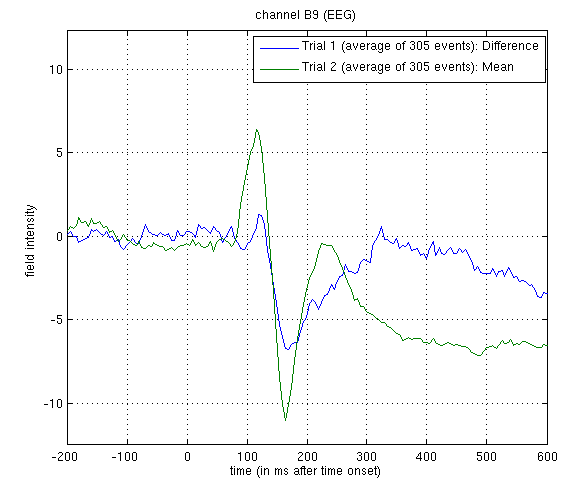
wmaceMdspm8_faces_run1.mat. The green line shows the average ERP evoked by faces and scrambled faces (at this occipitotemporal channel). A P1 and N1 are clearly seen. The blue line shows the differential ERP between faces and scrambled faces. The difference is small around the P1 latency, but large and negative around the N1 latency. The latter likely corresponds to the “N170” (Henson et al, 2003). We will try to localise the cortical sources of the P1 and N170 in Section [multimodal:eeg:3D].
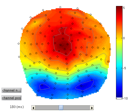
To see the topography of the differential ERP, click on Trial 1 again, press the “topography” icon button at the top of the window and scroll the latency from baseline to the end of the epoch. You should see a maximal difference around 180ms as in Figure 2 (possibly including a small delay of about 8ms for the CRT display to scan to the centre of the screen).
3D SPMs (Sensor Maps over Time) 
A feature of SPM is the ability to use Random Field Theory to correct for multiple statistical comparisons across N-dimensional spaces. For example, a 2D space representing the scalp data can be constructed by flattening the sensor locations (using the 2D layout we created earlier) and interpolating between them to create an image of \(M\times M\) pixels (when \(M\) is user-specified, eg \(M=32\)). This would allow one to identify locations where, for example, the ERP amplitude in two conditions at a given timepoint differed reliably across subjects, having corrected for the multiple t-tests performed across pixels. That correction uses Random Field Theory, which takes into account the spatial correlation across pixels (i.e, that the tests are not independent). This kind of analysis is described earlier in the SPM manual, where a 1st-level design is used to create the images for a given weighting across timepoints of an ERP/ERF, and a 2nd-level design can then be used to test these images across subjects.
Here, we will consider a 3D example, where the third dimension is time, and test across trials within the single subject. We first create a 3D image for each trial of the two types, with dimensions \(M\times M\times S\), where S=161 is the number of samples. We then take these images into an unpaired t-test across trials (in a 2nd-level model) to compare faces versus scrambled faces. We can then use classical SPM to identify locations in space and time in which a reliable difference occurs, correcting across the multiple comparisons entailed. This would be appropriate if, for example, we had no a priori knowledge where or when the difference between faces and scrambled faces would emerge4.
Select the “Convert to images” option in the “Other” menu in the SPM
main window, and select the aceMdspm8_faces_run1.mat file. You will
then be prompted for “output image dimensions”, for which you can accept
the default of 32 (leading to a \(32\times 32\) pixel space). It will then
ask whether you want to interpolate or mask out bad channels, for which
you select “interpolate” (though it will make no difference here because
there are no bad channels).
This will take some time as it writes out an image for each trial
(except rejected trials), in a new directory called
aceMdspm8_faces_run1, which will itself contain two subdirectories,
one for each trialtype. In each trialtype subdirectory there will be
image and header files for each non-rejected trial of that type, e.g,
trial0002.{hdr,img}. You can press “Display: images” to view one of
these images - it will have dimensions \(32\times 32\times 161\), with the
origin set at [16 18.6 41] (where 41 samples is 0ms), as in
Figure 3.
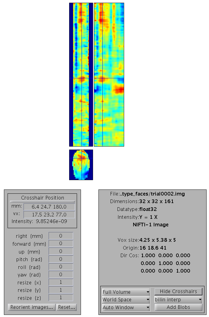
aceMdspm8_faces_run1.mat. The bottom image is a 2D x-y
space interpolated from the flattened electrode locations (at one point
in time). The two top images are sections through x and y respectively,
now expressed over time (vertical (z) dimension).Smoothing 
Note that you can also smooth these images in 3D (i.e, in space and time) by pressing “Smooth Images” from the “Others” pulldown menu. When you get the Batch Editor window, you can enter a smoothness of your choice (eg [9 9 20], or 9mm by 9mm by 20ms). Note that you should also change the default “Implicit masking” from “No” to “Yes”; this is to ensure that the smoothing does not extend beyond the edges of the topography.
As with fMRI, smoothing can improve statistics if the underlying signal has a smoothness close to the smoothing kernel (and the noise does not; the matched filter theorem). Smoothing may also be necessary if the final estimated smoothness of the SPMs (below) is not at least three times the voxel size; an assumption of Random Field Theory. In the present case, the data are already smooth enough (as you can check below), so we do not have to smooth further.
Stats 
To perform statistics on these images, first create a new directory, eg.
mkdir XYTstats.
Then press the “Specify 2nd level” button, to produce the batch editor
window again. Select the new XYTstats as the “Directory”, and
“two-sample t-test” (unpaired t-test) as the “Design”. Then select the
images for “group 1 scans” as all those in the subdirectory “type_faces”
(using right click, and “select all”) and the images for “group 2 scans”
as all those in the subdirectory “type_scrambled”. You might want to
save this batch specification, but then press “run”5.
This will produce the design matrix for a two-sample t-test.
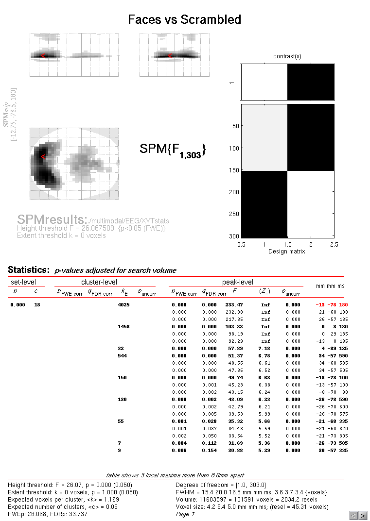
Then press “Estimate”, and when it has finished, press “Results” and define a new F-contrast as [1 -1]. Keep the default contrast options, but threshold at \(p<.05\) FWE corrected for the whole search volume and select “Scalp-Time” for the “Data Type”. Then press “whole brain”, and the Graphics window should now look like that in Figure 4.
This will reveal “regions” within the 2D sensor space and within the -200ms to 600ms epoch in which faces and scrambled faces differ reliably, having corrected for multiple F-tests across pixels and time. There are a number of such regions, but the largest has maxima at [-13 -78 180] and [21 -68 180], corresponding to left and right posterior sites at 180ms.
To relate these coordinates back to the original sensors, right-click in
some white space in the top half of the Graphics window, to get a menu
with various options. First select “goto global maxima”. The red cursor
should move to coordinates [-13, -78, 180]. (Note that you can also
overlap the sensor names on the MIP by selecting “display/hide
channels” - though it can get a bit crowded!). Then right-click again to
get the same menu, but this time select “go to nearest suprathreshold
channel”. You will be asked to select the original EEG/MEG file used to
create the SPM, which in this case is the aceMdspm8_faces_run1.mat
file. This should output in the Matlab window:
    spm_mip_ui: Jumped 4.25mm from [-13, -78, 180],
            to nearest suprathreshold channel (A15) at [ -8, -78, 180]
In other words, it is EEG channel “A15” that shows the greatest face/scrambled difference over the epoch (itself maximal at 180ms).
Note that an F-test was used because the sign of the difference reflects the polarity of the ERP difference, which is not of primary interest (and depends on the choice of reference). Indeed, if you plot the contrast of interest from the cluster maxima, you will see that the difference is negative for the first posterior, cluster but positive for the second, central cluster. This is consistent with the polarity of the differences in Figure 26.
If one had more constrained a priori knowledge about where and when the N170 would appear, one could perform an SVC based on, for example, a box around posterior channels and between 150 and 200ms poststimulus. See http://imaging.mrc-cbu.cam.ac.uk/meg/SensorSpm for more details.
If you go to the global maximum, then press “overlays”, “sections” and select the “mask.img” in the stats directory, you will get sections through the space-time image. A right click will reveal the current scalp location and time point. By moving the cursor around, you can see that the N170/VPP effects start to be significant (after whole-image correction) around 150ms (and may also notice a smaller but earlier effect around 100ms).
3D “imaging” reconstruction 
Here we will demonstrate a distributed source reconstruction of the N170 differential evoked response between faces and scrambled faces, using a grey-matter mesh extracted from the subject’s MRI, and the Multiple Sparse Priors (MSP) method in which multiple constraints on the solution can be imposed (Friston et al, 2008, Henson et al, 2009a).
Press the “3D source reconstruction” button, and press the “load” button
at the top of the new window. Select the wmaceMdspm8_faces_run1.mat
file and type a label (eg "N170 MSP") for this analysis7.
Press the “MRI” button, select the smri.img file within the sMRI
sub-directory, and select “normal” for the cortical mesh.
The “imaging” option corresponds to a distributed source localisation, where current sources are estimated at a large number of fixed points (8196 for a “normal” mesh here) within a cortical mesh, rather than approximated by a small number of equivalent dipoles (the ECD option). The imaging approach is better suited for group analyses and (probably) for later-occuring ERP components. The ECD approach may be better suited for very early sensory components (when only small parts of the brain are active), or for DCMs using a small number of regions (Kiebel et al, 2006).
The first time you use a particular structural image for 3D source
reconstruction, it will take some time while the MRI is segmented (and
normalisation parameters determined). This will create in the sMRI
directory the files y_smri.nii and smri_seg8.mat for normalisation
parameters and 4 GIfTI (.gii) files defining the cortical mesh, inner
skull, outer skull and scalp surface.
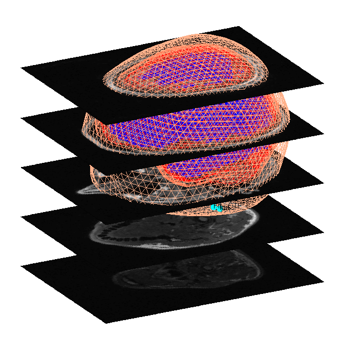
When meshing has finished, the cortex (blue), inner skull (red), outer
skull (orange) and scalp (pink) meshes will be shown in the Graphics
window with slices from the sMRI image, as shown in
Figure 5. This makes it possible to
visually verify that the meshes fit the original image well. The field
D.inv{1}.mesh field will be updated in MATLAB . Press “save” in top
right of window to update the corresponding mat file on disk.
Both the cortical mesh and the skull and scalp meshes are not created directly from the segmented MRI, but rather are determined from template meshes in MNI space via inverse spatial normalisation (Mattout et al, 2007).
Press the “Co-register” button. You will first be asked to select at least 3 fiducials from a list of points in the EEG dataset (from Polhemus file): by default, SPM has already highlighted what it thinks are the fiducials, i.e, points labelled “nas” (nasion), “lpa” (left preauricular) and “rpa” (right preauricular). So just press “ok”.
You will then be asked for each of the 3 fiducial points to specify its
location on the MRI images. This can be done by selecting a
corresponding point from a hard-coded list (“select”). These points are
inverse transformed for each individual image using the same deformation
field that is used to create the meshes. The other two options are
typing the MNI coordinates for each point (“type”) or clicking on the
corresponding point in the image (“click”). Here, we will type
coordinates based on where the experimenter defined the fiducials on the
smri.img. These coordinates can be found in the smri_fid.txt file
also provided. So press “type” and for “nas”, enter [0 91 -28]; for
“lpa” press “type” and enter [-72 4 -59]; for “rpa” press “type” and
enter [71 -6 -62]. Finally, answer “no” to “Use headshape points?” (in
theory, these headshape points could offer better coregistration, but in
this dataset, the digitised headshape points do not match the warped
scalp surface very well, as noted below, so just the fiducials are used
here).
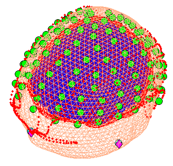
This stage coregisters the EEG sensor positions with the structural MRI and cortical mesh, via an approximate matching of the fiducials in the two spaces, followed by a more accurate surface-matching routine that fits the head-shape function (measured by Polhemus) to the scalp that was created in the previous meshing stage via segmentation of the MRI. When coregistration has finished, a figure like that in Figure 6 will appear in the top of the Graphics window, which you can rotate with the mouse (using the Rotate3D MATLAB Menu option) to check all sensors. Finally, press “save” in top right of window to update the corresponding mat file on disk.
Note that for these data, the coregistration is not optimal, with several EEG electrodes appearing inside the scalp. This may be inaccurate Polhemus recording of the headshape or inaccurate surface matching for the scalp mesh, or “slippage” of headpoints across the top of the scalp (which might be reduced in future by digitising features like the nose and ears, and including them in the scalp mesh). This is not actually a problem for the BEM calculated below, however, because the electrodes are re-projected to the scalp surface (as a precaution).
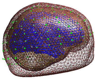
Press “Forward Model”, and select “EEG BEM”. The first time you do this,
there will be a lengthy computation and a large file smri_EEG_BEM.mat
will be saved in the sMRI directory containing the parameters of the
boundary element model (BEM). In the Graphics window the BEM meshes will
be displayed with the EEG sensors marked with green asterisks as shown
(after rotating to a “Y-Z” view using MATLAB rotate tool) in
Figure 7. This display is the final
quality control before the model is used for lead field computation.
Press “Invert”, select “Imaging” (i.e, a distributed solution rather than DCM; Kiebel et al (2006)), select “yes” to include all conditions (i.e, both the differential and common effects of faces and scrambled faces) and then “Standard” to use the default settings.
By default the MSP method will be used. MSP stands for “Multiple Sparse Priors” (Friston et al. 2008a), and has been shown to be superior to standard minimum norm (the alternative IID option) or a maximal smoothness solution (like LORETA; the COH option) - see Henson et al (2009a). Note that by default, MSP uses a “Greedy Search” (GS) (Friston et al, 2008b), though the standard ReML (as used in Henson et al, 2007) can also be selected via the batch tool (this uses Automatic Relevance Determination - ARD).
The “Standard” option uses default values for the MSP approach (to customise some of these parameters, press “Custom” instead).
At the first stage of the inversion lead fields will be computed for all
the mesh vertices and saved in the file
SPMgainmatrix_wmaceMdspm8_faces_run1_1.mat. Then the actual MSP
algorithm will run and the summary of the solution will be displayed in
the Graphics window.
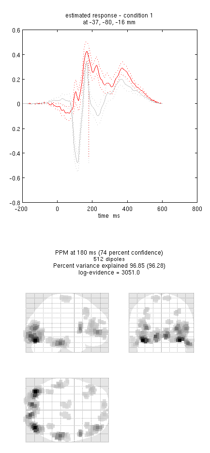
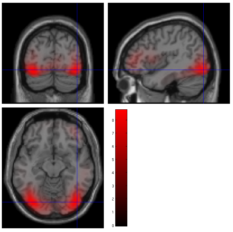
Press “save” to save the results. You can now explore the results via the 3D reconstruction window. If you type 180 into the box in the bottom right (corresponding to the time in ms) and press “mip”, you should see an output similar to Figure 8. This fit explains approx 96% of the data.
Note the hot-spots in bilateral posterior occipitotemporal cortex, bilateral mid-fusiform, and right lateral ventral temporal. The timecourses come from the peak voxel. The red curve shows the condition currently being shown (corresponding to the “Condition 1” toggle bar in the reconstruction window); the grey line(s) will show all other conditions. “Condition 1” is the differential evoked responses for faces vs scrambled; if you press the “condition 1” toggle, it will change to “Condition 2” (average evoked response for faces and scrambled faces), type “100”ms for the P100, then press “mip” again and the display will update (note the colours of the lines have now reversed from before, with red now corresponding to average ERP).
If you toggle back to “Condition 1” and press “movie”, you will see changes in the source strengths for the differential response over peristimulus time (from the limits 0 to 300ms currently chosen by default). If you press “render” you can get a very neat graphical interface to explore the data (the buttons are fairly self-explanatory).
You can also explore other inversion options, such as COH and IID (available for the “custom” inversion), which you will notice give more superficial solutions (a known problem with standard minimum norm approaches). To do this quickly (without repeating the MRI segmentation, coregistration and forward modelling), press the “new” button in the reconstruction window, which by default will copy these parts from the previous reconstruction.
In this final section we will concentrate on how to prepare source data for subsequent statistical analysis (eg with data from a group of subjects).
Press the “Window” button in the reconstruction window, enter “150 200” as the timewindow of interest and keep “0” as the frequency band of interest (0 means all frequencies). The Graphics window will then show the mean activity for this time/frequency contrast (top plot) and the contrast itself (bottom plot; note additional use of a Hanning window).
Then press “Image” and SPM will write 3D NIfTI images corresponding to the above contrast for each condition:
    wmaceMdspm8_faces_run1_1_t150_200_f_1.nii
    wmaceMdspm8_faces_run1_1_t150_200_f_2.nii
The last number in the file name refers to the condition number; the
number following the dataset name refers to the reconstruction number
(i.e. the number in red in the reconstruction window, i.e, D.val, here
1). The reconstruction number will increase if you create a new
inversion by pressing “new”.
The smoothed results for Condition 1 (i.e, the differential evoked response for faces vs scrambled faces) will also be displayed in the Graphics window, see Figure 9 (after moving the cursor to the right posterior hotspot), together with the normalised structural. Note that the solution image is in MNI (normalised) space, because the use of a canonical mesh provides us with a mapping between the cortex mesh in native space and the corresponding MNI space.
You can also of course view the image with the normal SPM “Display:image” option (just the functional image with no structural will be shown), and locate the coordinates of the “hotspots” in MNI space. Note that these images contain RMS (unsigned) source estimates (see Henson et al, 2007). Given that one has data from multiple subjects, one can create a NIFTI file for each. Group statistical analysis can the be implemented with eg. second level t-tests as described earlier in the chapter.
-
Re-referencing EEG to the mean over EEG channels is important for source localisation. Note also that if some channels are subsequently marked “bad” (see later), one should re-reference again, because bad channels are ignored in any localisation. ↩
-
You might need to change the full path to this text file inside the single quotes, depending on your current directory and the directory of the original data. ↩
-
When there are approximately equal numbers of trials in each condition, as here, it is probably safer to compute weights across all conditions, so as not to introduce artifactual differences between conditions. However, if one condition has fewer trials than the others, it is likely to be safer to estimate the weights separately for each condition, otherwise evoked responses in the rarer condition will be downweighted so as to become more similar to the more common condition(s). ↩
-
Note that the 2D location in sensor space for EEG will depend on the choice of montage. ↩
-
Note that we can use the default “nonsphericity” selections, i.e, that the two trial-types may have different variances, but are uncorrelated. ↩
-
The former likely corresponds to the “N170”, while the latter likely corresponds to the “VPP”, which may be two signs of the same effect, though of course these effects depend on the choice of reference. ↩
-
Note that no new M/EEG files are created during the 3D reconstruction; rather, each step involves updating of the cell-array field
D.inv, which will have one entry per analysis performed on that dataset (e.g,D.inv{1}in this case). ↩