Spatial preprocessing
Display
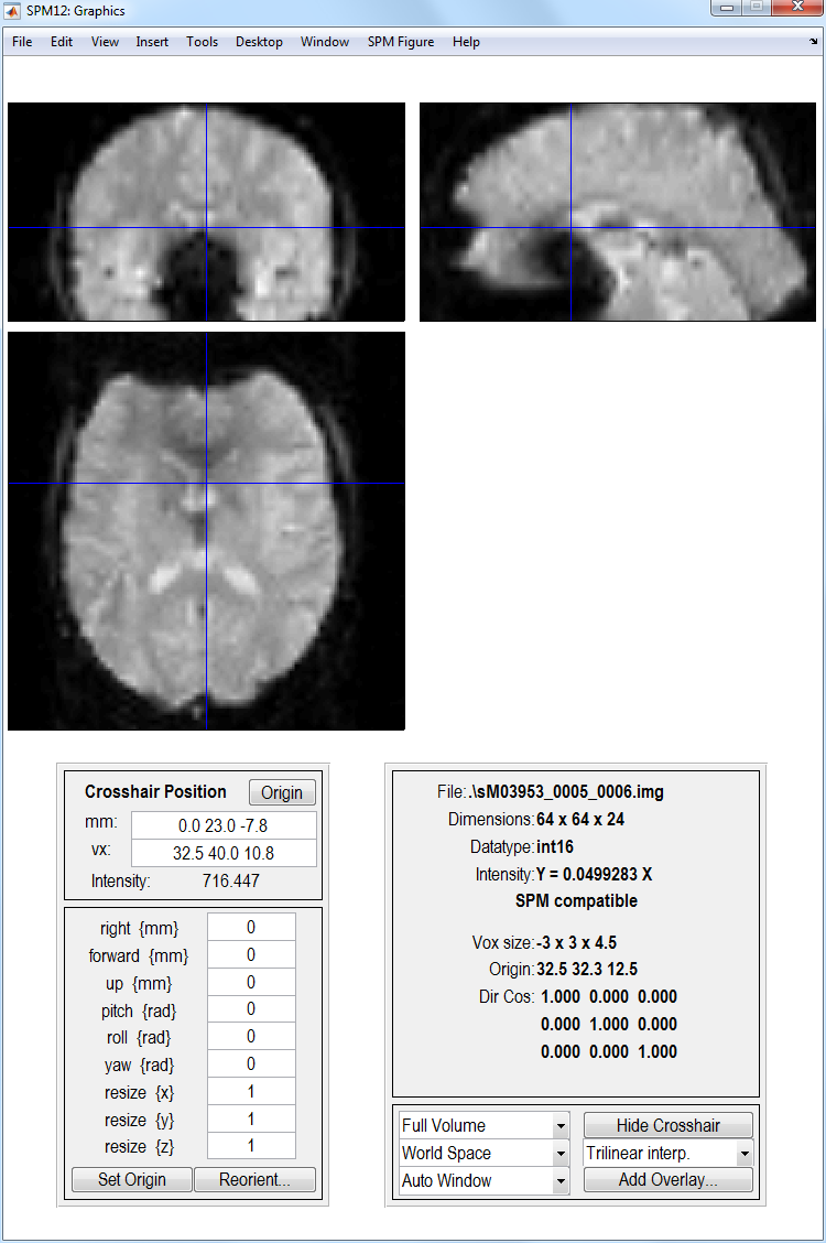
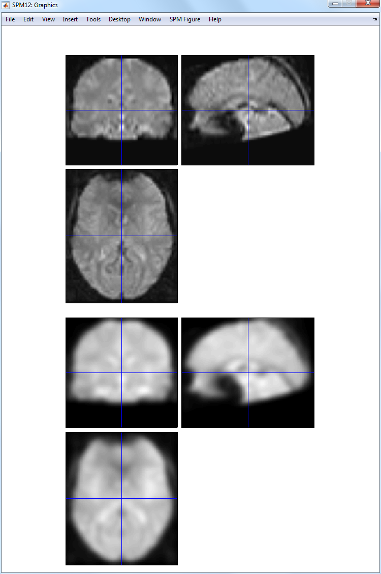
Display eg. the first functional image using the Display button. Note
orbitofrontal and inferior temporal drop-out and ghosting. This can be
seen more clearly by selecting Brighten from the Effects menu in the
Colours menu from the SPM Figure tab at the top of the Graphics
window.
Realignment
Under the spatial pre-processing section of the SPM base window select
Realign (Est & Res) from the
Realign pulldown menu. This will call up
a realignment job specification in the batch editor window. Then
-
Highlight data, select
New Session, then highlight the newly createdSessionoption. -
Select
Specify Filesand use the SPM file selector to choose all of your functional image volumes eg.sM03953_0005_*.img. You should select 351 volumes. -
Save the job file as eg.
DIR/jobs/realign.mat. -
Press the
Runbutton in the batch editor window (green triangle).
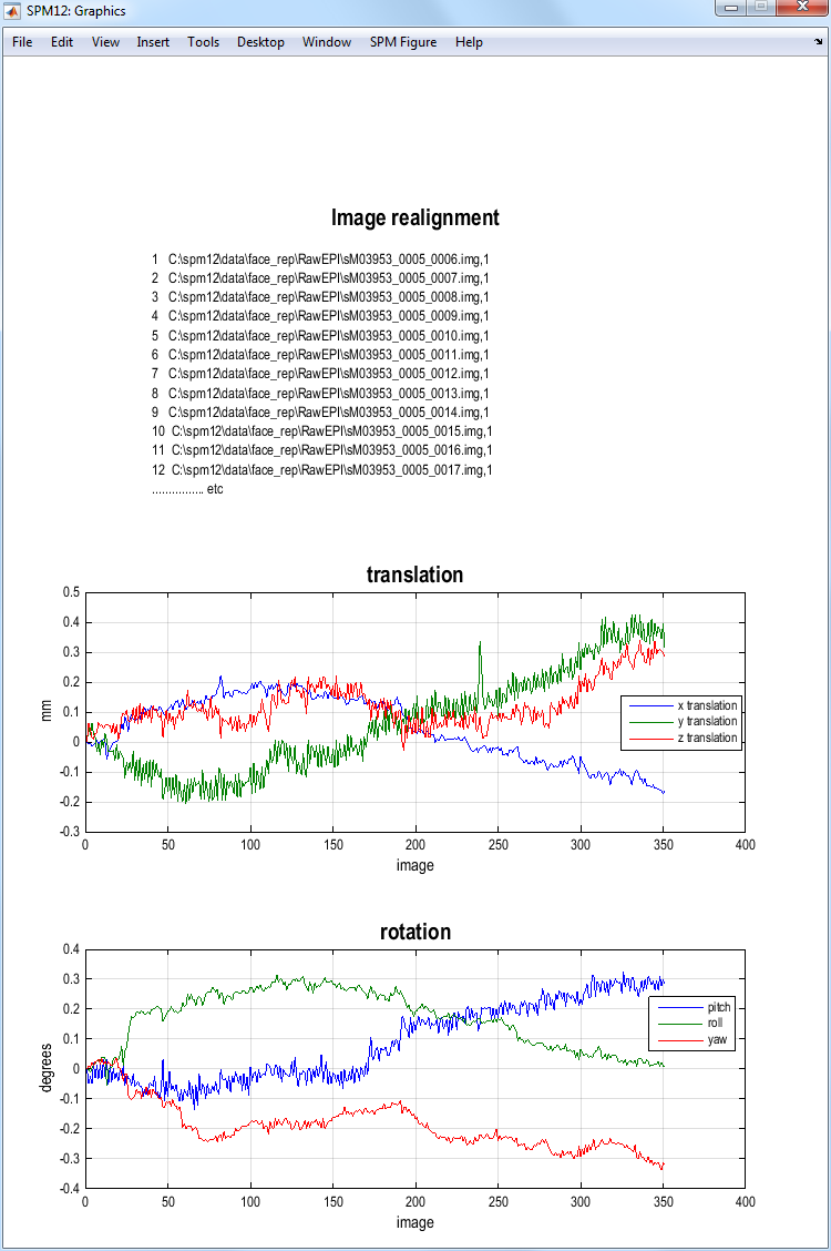
This will run the realign job which will write realigned images into the
folder where the functional images are. These new images will be
prefixed with the letter “r”. SPM will then plot the estimated time
series of translations and rotations. These data, the realignment
parameters, are also saved to a file eg. rp_sM03953_0005_0006.txt, so
that these variables can be used as regressors when fitting GLMs. This
allows movements effects to be discounted when looking for brain
activations.
SPM will also create a mean image eg. meansM03953_0005_0006.{hdr,img}
which will be used in the next step of spatial processing -
coregistration.
Slice timing correction
Press the Slice timing button. This will
call up the specification of a slice timing job in the batch editor
window. Note that these data consist of N=24 axial slices acquired
continuously with a TR=2s (ie TA = TR - TR/N, where TA is the time
between the onset of the first and last slice of one volume, and the TR
is the time between the onset of the first slice of one volume and the
first slice of next volume) and in a descending order (ie, most superior
slice was sampled first). The data however are ordered within the file
such that the first slice (slice number 1) is the most inferior slice,
making the slice acquisition order [24 23 22 ... 1].
-
Highlight
Dataand selectNew Sessions -
Highlight the newly create
Sessionsoption,Specify Filesand select the 351 realigned functional images using the filter^r.*. -
Select
Number of Slicesand enter24. -
Select
TRand enter2. -
Select
TAand enter1.92(or2 - 2/24). -
Select
Slice orderand enter24:-1:1. -
Select
Reference Slice, and enter12. -
Save the job as
slice_timing.matand press theRunbutton.
SPM will write slice-time corrected versions of the images with the prefix a in the
same folder as the functional data.
Coregistration
Select Coregister (Estimate) from the
Coregister pulldown menu. This will call up the specification of a
coregistration job in the batch editor window.
-
Highlight
Fixed Imageand then select the mean functional imagemeansM03953_0005_0006.img. -
Highlight
Moved Imageand then select the structural image eg.sM03953_0007.img. -
Press the
Savebutton and save the job ascoreg.job -
Then press the
Runbutton.
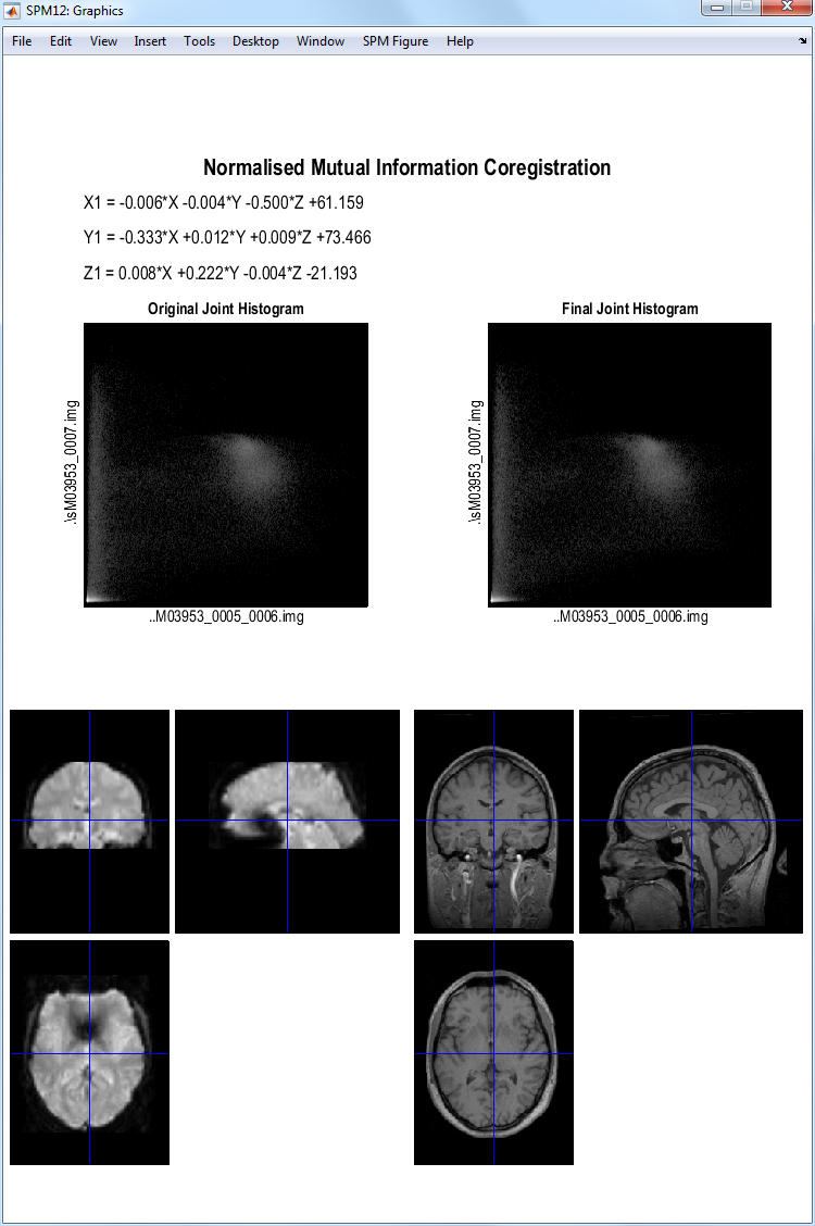
SPM will then implement a coregistration between the structural and
functional data that maximises the mutual information. The image
displayed below should then appear in the Graphics
window. SPM will have changed the header of the moved file, which in
this case is the structural image sM03953_0007.hdr.
Segmentation
Press the Segment button. This will call
up the specification of a segmentation job in the batch editor window.
Highlight the Volumes field in Data > Channels and then select the
subjects coregistered anatomical image eg. sM03953_0007.img. Change
Save INU corrected so that it contains Save INU corrected instead
of Save nothing. At the bottom of the list, select Forward in
Deformation Fields. Save the job file as segment.mat and then press
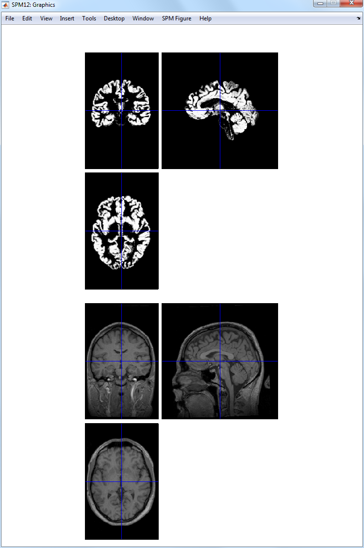
the Run button. SPM will segment the structural image using the
default tissue probability maps as priors. SPM will create, by default,
gray and white matter images and intensity nonuniformity corrected structural image.
These can be viewed using the CheckReg facility as described in the
previous section 1.
SPM will also write a spatial normalisation deformation field file eg.
y_sM03953_0007.nii file in the original structural folder. This
will be used in the next section to normalise the functional data.
Normalise
Select Normalise (Write) from the
Normalise pulldown menu. This will call
up the specification of a normalise job in the batch editor window.
-
Highlight
Data, selectNew Subject. -
Open
Subject, highlightDeformation fieldand select they_sM03953_0007.niifile that you created in the previous section. -
Highlight
Images to writeand select all of the slice-time corrected, realigned functional imagesarsM*.img. Note: This can be done efficiently by changing the filter in the SPM file selector to^ar.*. You can then right click over the listed images, chooseSelect all. You might also want to select the mean functional image created during realignment (which would not be affected by slice-time correction), i.e, themeansM03953_0005_006.img. Then pressDone. -
Open
Writing Options, and changeVoxel sizesfrom [2 2 2] to [3 3 3]2. -
Press
Save, save the job as normalise.mat and then press theRunbutton.
SPM will then write spatially normalised versions of the images to the folder containing the functional data.
These files have the prefix w.
If you wish to superimpose a subject’s functional activations on their own anatomy 3 you will also need to apply the spatial normalisation parameters to their (intensity nonuniformity corrected) anatomical image. To do this
-
Select
Normalise (Write), highlightData, selectNew Subject. -
Highlight
Deformation field, select they_sM03953_0007.niifile that you created in the previous section, pressDone. -
Highlight
Images to Write, select the intensity nonuniformity corrected structural eg.msM03953_0007.nii, pressDone. -
Open
Writing Options, select voxel sizes and change the default [2 2 2] to [1 1 1] which better matches the original resolution of the images [1 1 1.5]. -
Save the job as
norm_struct.matand pressRunbutton.
Smoothing
Press the Smooth button 4. This will
call up the specification of a smooth job in the batch editor window.
-
Select
Images to Smoothand then select the spatially normalised volumes created in the last section eg.war*.img. -
Save the job as smooth.mat and press
Runbutton.
This will smooth the data by (the default) 8mm in each direction, the default smoothing kernel width.
-
Segmentation can sometimes fail if the source (structural) image is not close in orientation to the MNI templates. It is generally advisable to manually orient the structural to match the template (ie MNI space) as close as possible by using the “Display” button, adjusting x/y/z/pitch/roll/yaw, and then pressing the “Reorient” button. ↩
-
This step is not strictly necessary. It will write images out at a resolution closer to that at which they were acquired. This will speed up subsequent analysis and is necessary, for example, to make Bayesian fMRI analysis computationally efficient. ↩
-
Beginners may wish to skip this step, and instead just superimpose functional activations on an “canonical structural image”. ↩
-
The smoothing step is unnecessary if you are only interested in Bayesian analysis of your functional data. ↩