Voxel-Based Morphometry
For MSc Advanced Neuroimaging students
These notes were originally written for the MSc in Advanced Neuroimaging students at UCL.
Learning Objectives
-
Increase familiarity with using MATLAB and the SPM12 software.
-
Learn about the image features that voxel-based morphometry compares and how they are derived.
-
Understand some of the limitations of the method and how to be more cautious when reading papers.
Data and SPM
Data is provided for the MSc students, but others may wish to use their own, or download datasets from (e.g.) http://www.brain-development.org/.
To save time, students are advised to copy all the folders containing the example dataset from S:\IoN_Education_PGTstudents\ANIWorkshops\P4\P4MVW1 to somewhere in the local workspace. This would save time, because copying would be very slow if everyone tries to do it at the same time. Please don’t work in the original example dataset folder (i.e., work on your copy) because this messes thing up for other students.
The data provided are a selection of T1-weighted scans from the freely available IXI dataset, available via http://www.brain-development.org/. Note that the scans were acquired in the sagittal orientation, but a matrix in the NIfTI headers encodes this information so SPM can treat them as axial.
SPM12 appears to have been installed in the S:\IoN_Education_PGTstudents\ANIWorkshops\Software\spm12 folder, so there is no need to download it now.
The overall plan will be to
-
Start up SPM.
-
Check that the images are in a suitable format (Check Reg and Display buttons).
-
Segment the images, to identify grey and white matter (using the Segment button). Grey matter will eventually be warped to MNI space. This step also generates “imported” images, which will be used in the next step.
-
Estimate the deformations that best align the images together by iteratively registering the imported images with their average (SPMToolsShoot ToolsRun Shooting (create Templates)).
-
Generate spatially normalised and smoothed Jacobian scaled grey matter images, using the deformations estimated in the previous step (SPMToolsShoot ToolsWrite Normalised).
-
Do some statistics on the smoothed images (Basic models, Estimate and Results options).
The tutorial will use SPM12, which is is available from http://www.fil.ion.ucl.ac.uk/spm/, and is the latest SPM software release. SPM runs in the MATLAB package, which is worth learning how to program a little if you ever plan to do any imaging research.
Older SPM versions
Older versions are SPM8, SPM5, SPM2, SPM99, SPM96 and SPM91 (SPMclassic). Anything before SPM5 is considered ancient, and any good manuscript reviewer will look down their noses at studies done using ancient software versions.
Start MATLAB. SPM is started from within MATLAB by typing
or (eg)This will pop open a bunch of windows. The top-left one is the one with the buttons. The Batch button on this window will call the batching system used in this workshop.
Can’t find SPM?
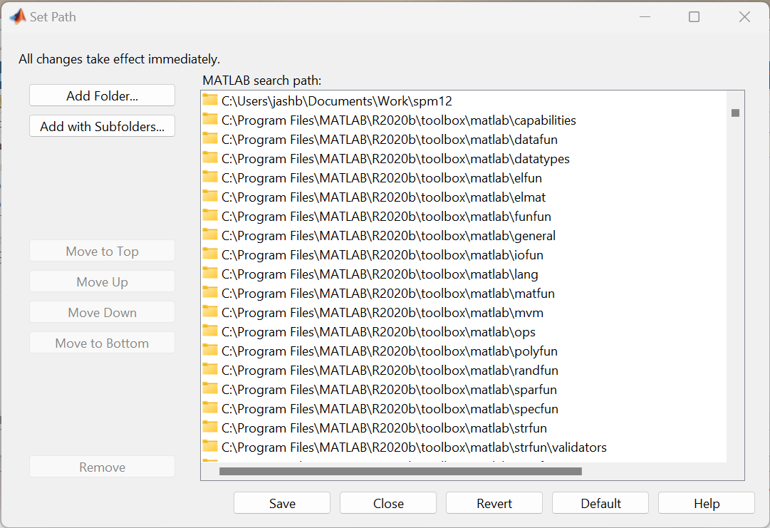
If MATLAB can’t find spm, then it probably needs the search path to be correctly set. Find and click the Set Path button in the MATLAB user interface. This will give you a window that allows you to tell MATLAB where to find the SPM12 software.
More advanced users could use the path command to do this.
You are advised to change to the directory where you have the data, as this makes it much easier to select files for displaying or processing. You can do this using MATLAB’s cd command, although there is an option on the SPM user interface that allows you to CD (find the pulldown saying Utils).
Image file format
SPM requires the image data in a suitable format. The example data are already in NIfTI format, but most scanners produce images in DICOM format. For other data, the DICOM button of SPM can be used to convert many versions of DICOM into NIfTI format, which SPM (and a number of other packages, eg FSL, MRIcron etc) can use. There are two main forms of NIfTI:
-
.hdrand.imgfiles, which appear superficially similar to the older ANALYZE format. The .img file contains the actual image data, and the .hdr contains the information necessary for programs to understand it. -
.niifiles, which combines all the information into one file.
Images consist of arrays of voxels, which are like pixels, but in 3D. Voxels are numbers, which can be represented by various different datatypes. Integer datatypes can only encode a limited range of values, and are usually used to save some disk space. For example, the uint8 datatype can only encode integer values from 0 to 255, and the int16 datatype can only encode values from -32768 to 32767. For this reason, there is also a scale-factor (and sometimes a constant term) saved in the headers in order to make the values more quantitative. For example, a uint8 datatype may be used to save an image of probabilities, which can take values from 0.0 to 1.0. This would involve a scale-factor in the header of 1/255.
NIfTI images can consist of single 3D volumes, but 4D or even 5D images are possible. For SPM5 onwards, the 4D images may have an additional .mat file.
Check Reg button
For MSc Advanced Neuroimaging students
MSc Advanced Neuroimaging students should work with the IXI scans from the examples folder.
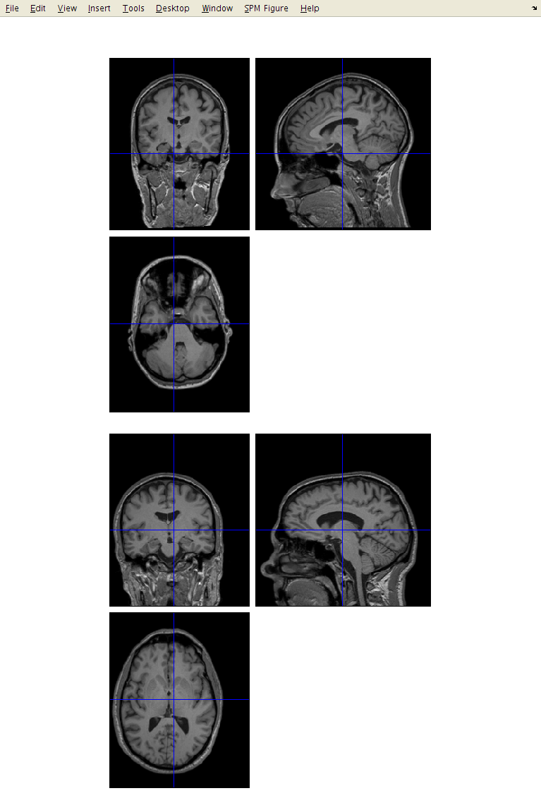
Click the Check Reg button and select one (or more) of the original scans, as well as the canonical\avg152T1.nii file in the SPM12 release. This shows the relative positions of the images, as understood by SPM. Note that if you click the right mouse button on one of the images, you will be shown a menu of options, which you may wish to try. If images need to be rotated or translated (shifted), then this can be done using the Display button. Before you begin, each image should be approximately aligned within about 5 cm and about 20 degrees of the template data released with SPM.
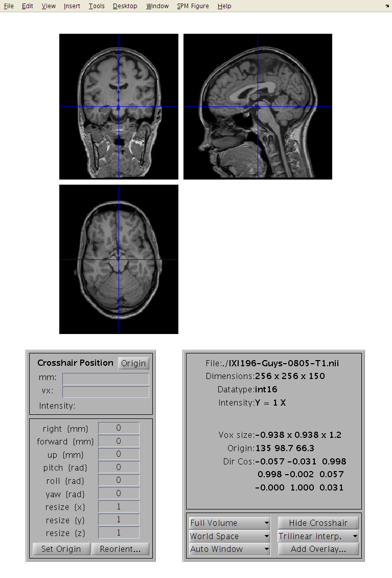
Display button
Click the Display button, and select an image. This should show you three slices through the image. If you have the images in the correct format, then:
-
The top-left image is coronal with the top (superior) of the head displayed at the top and the left shown on the left. This is as if the subject is viewed from behind.
-
The bottom-left image is axial with the front (anterior) of the head at the top and the left shown on the left. This is as if the subject is viewed from above.
-
The top-right image is sagittal with the front (anterior) of the head at the left and the top of the head shown at the top. This is as if the subject is viewed from the left.
You can click on the sections to move the cross-hairs and see a different view of the 3D image. Below the three views are a couple of panels. The one on the left gives you information about the position of the cross-hair and the intensity of the image below it. The positions are reported in both mm and voxels. The coordinates in mm represent the orientation within some Cartesian coordinate system (e.g., scanner coordinate system, or MNI space). The vx coordinates indicate which voxel you are at (where the first voxel in the file has coordinate 1,1,1). Clicking on the horizontal bar, above, will move the cursor to the origin (mm coordinate 0,0,0), which should be close(ish) to the anterior commissure (AC). The intensity at the point in the image below the cross-hairs is obtained by interpolation of the neighbouring voxels. This means that for a binary image, the intensity may not be shown as exactly 0 or 1.
Below this are a number of boxes that allow the image to be re-oriented and shifted. If you click on the AC, you can see its mm coordinates. The objective is to move this point to a position close to 0,0,0. To do this, you would translate the images by minus the mm coordinates shown for the AC. These values would be entered into the right {mm}, forward {mm} and up {mm} boxes.
If rotations are needed, they can be entered into rotation boxes. Notice that the angles are specified in radians, so a rotation of 90 degrees would be entered as 1.5708 or as pi/2. When entering rotations around different axes, the result can be a bit confusing, so some trial and error may be needed. Note that pitch refers to rotations about the x axis, roll is for rotations about the y axis and yaw is for rotations about the z axis.
Pitch, roll and yaw
Note that in aeronautics, pitch, roll and yaw would be defined differently, but that is because they use a different labelling of their axes.
To actually change the header of the image, you can use the Reorient images… button. This allows you to select multiple images, which would all be rotated and translated in the same way.
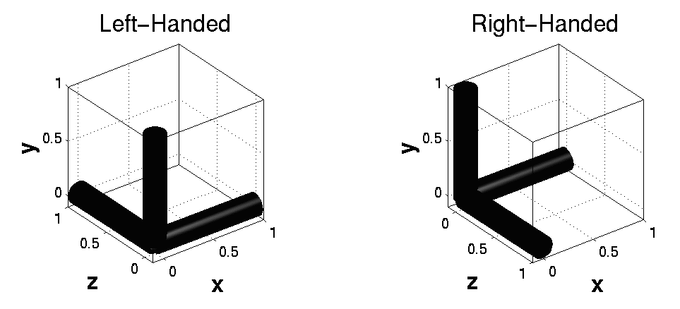
The panel on the right shows various pieces of information about the image being displayed. Below this lot is some positional and voxel size information. Note that the first element of the voxel sizes may be negative. This indicates whether there is a reflection between the coordinate system of the voxels and the mm coordinate system. One of them is right-handed, whereas the other is left-handed.
Another option allows the image to be zoomed to a region around the cross-hair. The effects of changing the interpolation are most apparent when the image is zoomed up. Also, if the original image was collected in a different orientation, then the image can be viewed in Native Space (as opposed to World Space), to show it this way.