Modelling categorical responses
Onset times
Before setting up the design matrix we must first load the Stimulus
Onsets Times (SOTs) into MATLAB . SOTs are stored in the sots.mat file
in a cell array such that eg. sot{1} contains stimulus onset times in
TRs for event type 1, which is N1. Event-types 2, 3 and 4 are N2, F1 and
F2.1
- At the MATLAB command prompt type
load sots
Model specification
Now press the Specify 1st-level button.
This will call up the specification of a fMRI specification job in the
batch editor window. Then
-
For
Directory, select thecategoricalfolder (directory) you created earlier, -
In the
Timing parametersoption, -
Highlight
Units for designand selectScans, -
Highlight
Interscan intervaland enter2, -
Highlight
Microtime resolutionand enter24, -
Highlight
Microtime onsetand enter12. These last two options make the creating of regressors commensurate with the slice-time correction we have applied to the data, given that there are 24 slices and that the reference slice to which the data were slice-time corrected was the 12th (middle slice in time). -
Highlight
Data and Designand selectNew Subject/Session. -
Highlight
Scansand use SPM’s file selector to choose the 351 smoothed, normalised, slice-time corrected, realigned functional images ieswarsM.img. These can be selected easily using the^swar.*filter, and select all. Then pressDone. -
Highlight
Conditionsand selectNew condition2. -
Open the newly created
Conditionoption. HighlightNameand enterN1. HighlightOnsetsand entersot{1}. HighlightDurationsand enter0. -
Highlight
Conditionsand selectReplicate condition. -
Open the newly created
Conditionoption (the lowest one). HighlightNameand change toN2. HighlightOnsetsand entersot{2}. -
Highlight
Conditionsand selectReplicate condition. -
Open the newly created
Conditionoption (the lowest one). HighlightNameand change toF1. HighlightOnsetsand entersot{3}. -
Highlight
Conditionsand selectReplicate condition. -
Open the newly created
Conditionoption (the lowest one). HighlightNameand change toF2. HighlightOnsetsand entersot{4}. -
Highlight
Multiple Regressorsand select the realignment parameter filerp_sM03953_0005_0006.txtfile that was saved during the realignment preprocessing step in the folder containing the fMRI data3. -
Highlight
Factorial Design, selectNew Factor, open the newly createdFactoroption, highlightNameand enterFam, highlightLevelsand enter2. -
Highlight
Factorial Design, selectNew Factor, open the newly createdFactoroption, highlightNameand enterRep, highlightLevelsand enter 24. -
Open
Canonical HRFunderBasis Functions. SelectModel derivativesand selectTime and Dispersion derivatives. -
Highlight
Directoryand select theDIR/categoricalfolder you created earlier. -
Save the job as
categorical_spec.matand press theRunbutton.
SPM will then write an SPM.mat file to the DIR/categorical
folder. It will also plot the design matrix, as shown below
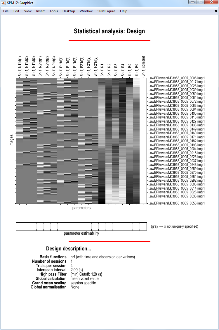
At this stage it is advisable to check your model specification using
SPM’s review facility which is accessed via the Review button. This
brings up a Design tab on the interactive window clicking on which
produces a pulldown menu. If you select the first item Design Matrix
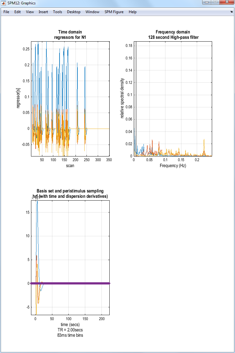
SPM will produce the image shown above. If you select Explore then
Session 1 then N1, SPM will produce the plots shown below.
Model estimation
Press the Estimate button. This will call
up the specification of an fMRI estimation job in the batch editor
window. Then
-
Highlight the
Select SPM.matoption and then choose theSPM.matfile saved in theDIR/categoricalfolder. -
Save the job as
categorical_est.joband pressRunbutton.
SPM will write a number of files into the selected folder including
an SPM.mat file.
Inference for categorical design
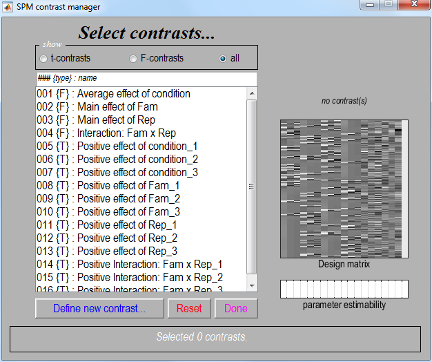
Press “Results” and select the SPM.mat file from DIR/categorical. This
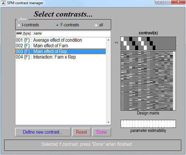
will again invoke the contrast manager. Because we specified that our
model was using a “Factorial design” a number of contrasts have been
specified automatically, as shown below.
-
Select contrast number 5. This is a t-contrast
Positive effect of condition_1This will show regions where the average effect of presenting faces is significantly positive, as modelled by the first regressor (hence the_1), the canonical HRF. PressDone. -
Apply masking ? [None/Contrast/Image]
- Specify
None.
- Specify
-
p value adjustment to control: [FWE/none]
- Select
FWE.
- Select
-
Corrected p value(family-wise error)
- Accept the default value,
0.05
- Accept the default value,
-
Extent threshold {voxels} [0]
- Accept the default value,
0.
- Accept the default value,
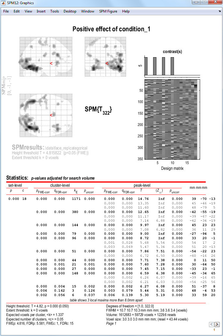
SPM will then produce the MIP shown below.
Statistical tables
To get a summary of local maxima, press the whole brain button in the
p-values section of the interactive window. This will list all clusters
above the chosen level of significance as well as separate
(\(>\)8mm apart) maxima within a cluster, with details of
significance thresholds and search volume underneath.
The columns in volume table show, from right to left:
-
x, y, z (mm): coordinates in MNI space for each maximum.
-
peak-level: the chance (p) of finding (under the null hypothesis) a peak with this or a greater height (T- or Z-statistic), corrected (FWE or FDR) / uncorrected for search volume.
-
cluster-level: the chance (p) of finding a cluster with this many(ke) or a greater number of voxels, corrected (FWE or FDR) / uncorrected for search volume.
-
set-level: the chance (p) of finding this (c) or a greater number of clusters in the search volume.
Right-click on the MIP and select goto global maximum. The cursor will
move to [39 -70 -14]. You can view this activation on the subject’s
normalised, intensity nonuniformity corrected structural (wmsM03953_0007i̇mg), which gives
best anatomical precision, or on the normalised mean functional
(wmeansM03953_0005_0006.nii), which is closer to the true data and
spatial resolution (including distortions in the functional EPI data).
If you select plot and choose Contrast of estimates and 90% C.I
(confidence interval), and select the Average effect of condition
contrast, you will see three bars corresponding to the parameter
estimates for each basis function (summed across the 4 conditions). The
BOLD impulse response in this voxel loads mainly on the canonical HRF,
but also significantly (given that the error bars do not overlap zero)
on the temporal and dispersion derivatives (see next Chapter).
F-contrasts
To assess the main effect of repeating faces, as characterised by both the hrf and its derivatives, an F-contrats is required. This is really asking whether repetition changes the shape of the impulse response (e.g, it might affect its latency but not peak amplitude), at least the range of shapes defined by the three basis functions. Because we have told SPM that we have a factorial design, this required contrast will have been created automatically - it is number 3.
-
Press
Resultsand select theSPM.matfile in theDIR/categoricalfolder. -
Select the
F-contrasttoggle and the contrast number 3, as shown in the next image. PressDone. -
Apply masking ? [None/Contrast/Image].
-
Specify
Contrast. -
Select contrast 5 -
Positive effect of condition_1(the T-contrast of activation versus baseline, collapsed across conditions, that we evaluated above)
-
-
uncorrected mask p-value ?
- Change to
0.001.
- Change to
-
nature of mask?
- Select
inclusive.
- Select
-
p value adjustment to control: [FWE/none]
- Select
none.
- Select
-
threshold (F or p value)
- Accept the default value,
0.001.
- Accept the default value,
-
Extent threshold {voxels} [0]
- Accept the default value,
0.
- Accept the default value,
A MIP should then appear, the top half of which should look like the figure below.
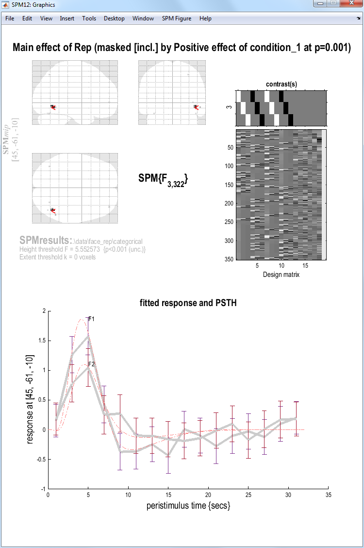
Note that this contrast will identify regions showing any effect of
repetition (e.g, decreased or increased amplitudes) within those
regions showing activations (on the canonical HRF) to faces versus
baseline (at p\(<\).05 uncorrected). Select “goto global max”, which is in
right ventral temporal cortex [42 -64 -8].
If you press plot and select Event-related responses, then F1, then
fitted response and PSTH, you will see the best fitting linear
combination of the canonical HRF and its two derivatives (thin red
line), plus the “selectively-averaged” data (peri-stimulus histogram,
PSTH), based on an FIR refit (see next Chapter). If you then select the
hold button on the Interactive window, and then plot and repeat the
above process for the F2 rather than F1 condition, you will see two
estimated event-related responses, in which repetition decreases the
peak response (ie F2\(<\)F1), as shown in the figure above.
You can explore further F-contrasts, which are a powerful tool once you
understand them. For example, the MIP produced by the “Average effect of
condition” F-contrast looks similar to the earlier T-contrast, but
importantly shows the areas for which the sums across conditions of the
parameter estimates for the canonical hrf and/or its temporal
derivative and/or its dispersion derivative are different from zero
(baseline). The first row of this F-contrast ([1 0 0 1 0 0 1 0 0 1 0
0]) is also a two-tailed version of the above T-contrast, ie testing
for both activations and deactivations versus baseline. This also means
that the F-contrasts [1 0 0 1 0 0 1 0 0 1 0 0] and [-1 0 0 -1 0 0 -1
0 0 -1 0 0] are equivalent. Finally, note that an F- (or t-) contrast
such as [1 1 1 1 1 1 1 1 1 1 1], which tests whether the mean of the
canonical hrf AND its derivatives for all conditions are different from
(larger than) zero is not sensible. This is because the canonical hrf
and its temporal derivative may cancel each other out while being
significant in their own right. The basis functions are really quite
different things, and need to represent separate rows in an F-contrast.
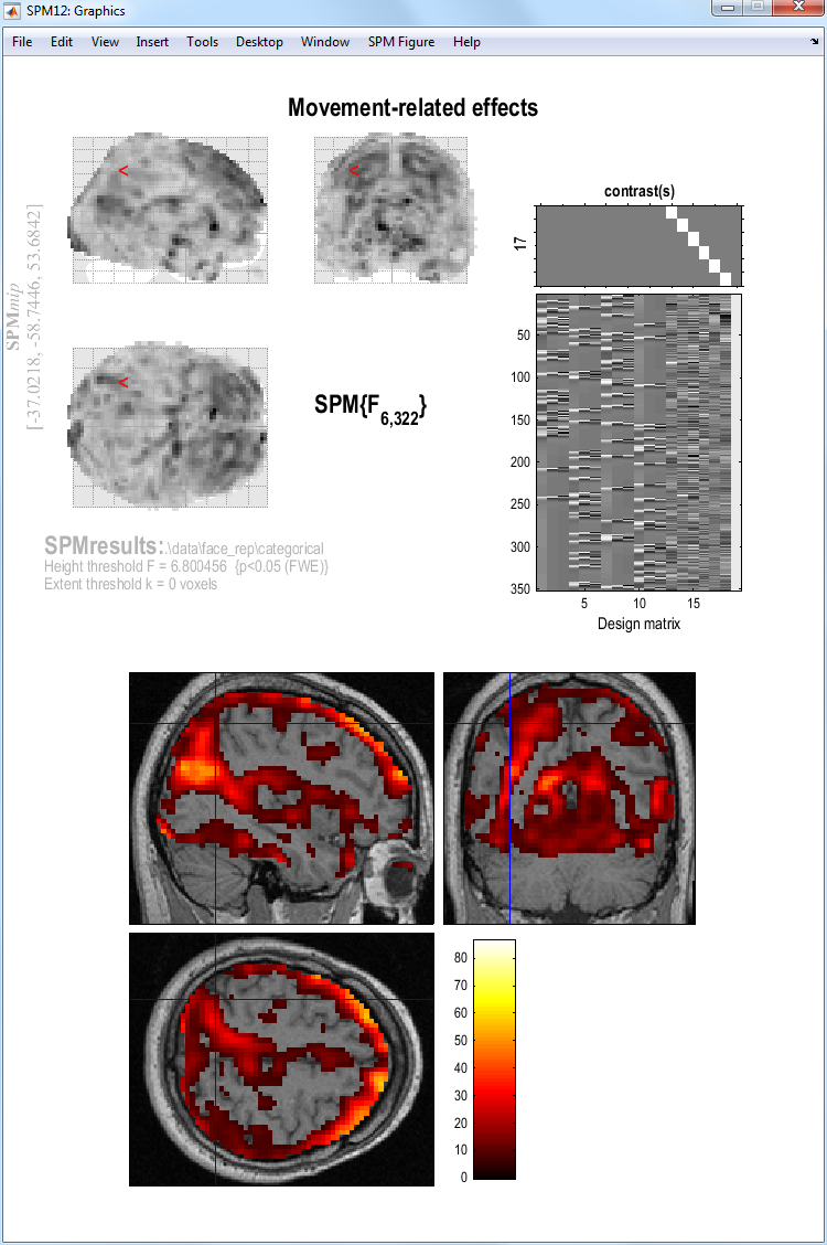
F-contrasts for testing effects of movement
To assess movement-related activation
-
Press
Results, select theSPM.matfile, selectF-contrastin the Contrast Manager. Specify e.g.Movement-related effects(name) and in thecontrasts weights matrixwindow, or1:12 19in thecolumns for reduced designwindow. -
Submit and select the contrast, specify
Apply masking?(none),corrected height threshold(FWE), andcorrected p-value(accept default). -
When the MIP appears, select
sectionsfrom theoverlayspulldown menu, and select the normalised structural image (wmsM03953_0007.nii).
You will see there is a lot of residual movement-related artifact in the data (despite spatial realignment), which tends to be concentrated near the boundaries of tissue types (eg the edge of the brain; see below). (Note how the MIP can be misleading in this respect, since though it appears that the whole brain is affected, this reflects the nature of the (X-ray like) projections onto each orthogonal view; displaying the same data as sections in 3D shows that not every voxel is suprathreshold.) Even though we are not interested in such artifact, by including the realignment parameters in our design matrix, we “covary out” (linear components) of subject movement, reducing the residual error, and hence improve our statistics for the effects of interest.
-
Unlike previous analyses of these data in SPM99 and SPM2, we will not bother with extra event-types for the (rare) error trials. ↩
-
It is also possible to enter information about all of the conditions in one go. This requires much less button pressing and can be implemented by highlighting the “Multiple conditions” option and then selecting the
all-conditions.matfile, which is also provided on the webpage. ↩ -
It is also possible to enter regressors one by one by highlighting “Regressors” and selecting “New Regressor” for each one. Here, we benefit from the fact that the realignment stage produced a text file with the correct number of rows (351) and columns (6) for SPM to add 6 regressors to model (linear) rigid-body movement effects. ↩
-
The order of naming these factors is important - the factor to be specified first is the one that “changes slowest” ie. as we go through the list of conditions N1, N2, F1, F2 the factor “repetition” changes every condition and the factor “fame” changes every other condition. So “Fam” changes slowest and is entered first. ↩