Convolution modelling of M/EEG data¶

This chapter demonstrates an example of first-level modelling of M/EEG data using the convolution GLM introduced in (V. Litvak et al., 2013)¹. The example is based on a workshop held by B. Spitzer in 2015 (see on GitHub) and reproduces the results presented in (B. Spitzer et al., 2016)² for a single subject.

Overview¶

The experimental setup involved presenting visual, auditory, and somatosensory stimuli to subjects in a supramodal integration task. In this example, we aim to investigate the EEG response to different modalities of sensory stimuli, specifically visual, auditory, and tactile pulses. To compare the responses, we want to capture the average event-related response for each modality across trials. However, conventional methods of averaging across trials to generate an event-related potential are not suitable for this experiment because the delay between consecutive pulses can be as short as 100 ms, resulting in overlap of the responses over time. Therefore, we need to employ more elaborate techniques to disentangle – more precisely, to deconvolve – the responses over time.

The convolution GLM provides a way to deconvolve the responses using a standard GLM with some particular regressors in its design matrix. In convolution GLM, the rows of the design matrix represent time, and the response regressors are obtained by convolving event indicators with a basis set. This allows us to model the possible overlap between responses to consecutive stimulis. Here, we will see how to parameterize the basis set and its duration, as well as the events, to perform convolution modelling in SPM.

Preliminary steps¶

GUIScript

The data provided (here) for this tutorial have already been preprocessed. However, there are still a few preparation steps required: we need to re-reference, filter, and mark artefacts.

Setup the workspace

In this tutorial, we will have a standard folder layout for SPM analysis:

+   the original data will be in a `data/` folder
+   the intermediate and final datasets will be in an `analysis/`
    folder

clear;
cwd      = pwd;
workpath = fullfile(cwd, 'analysis');
datapath = fullfile(cwd, 'data');
spm_mkdir(workpath);

Then, warm up SPM:

spm('defaults', 'eeg');

Prepare the data

The data has already been converted to SPM and downsampled to 128Hz. This is single subject data with the following name and prefix (“d” for downsampled). Download the files and put them in the data folder. We then move them programmatically to the analysis folder (this makes sure that the original data files are kept intact).
```
name   = 'pil02';
prefix = 'd';
copyfile(fullfile(datapath, [prefix name '.*']), workpath);
```

Rereferencing¶

Lets reference the EEG channels against the common average.

GUIScript

Start SPM in EEG mode.
Click on “Prepare (batch)” in the upper panel of the main SPM window,
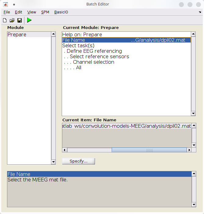
Configure the “Prepare” batch:
- Under file name, select “dpil02.mat”,
- Under “Select task(s)”, select “EEG referencing” and leave defaults settings to reference against the average.

First, load the data:

D = spm_eeg_load(fullfile(workpath, [prefix name '.mat']));

Then, define the transform to apply to make the new (rereferenced) montage:

tra             = zeros(66, D.nchannels);
tra(1:64, 1:64) = eye(64) - 1/64;
tra(65, 67:68)  = [1 -1];
tra(66, 65:66)  = [1 -1];

In addition we need to specify that EOG channels are bipolar, thus only the difference is of interest. Finally, use spm_eeg_montage to transform the data:

S = []; 

S.D                = fullfile(workpath, D.fname);
S.montage.tra      = tra;
S.montage.labelnew = [D.chanlabels(1:64) 'VEOG' 'HEOG'];
S.montage.labelorg = D.chanlabels;
S.keepothers       = 0;

[D, montage] = spm_eeg_montage(S);

prefix = ['M' prefix];

Filtering¶

We high-pass filter the data at 0.5Hz:

GUIScript

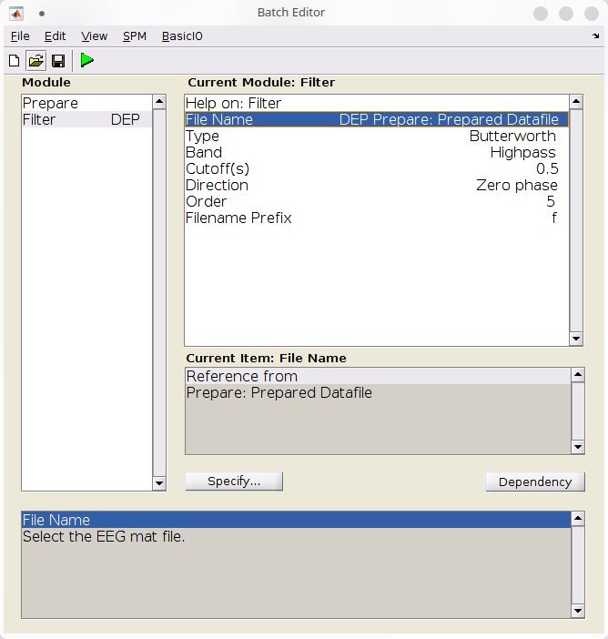
Add a “filter” batch (SPM >M/EEG >Preprocessing >Filter),
Configure a 5th-order Butterworth highpass filter at \(0.5Hz\):
- Under file name, use the dependency button to refer to the file produced by the previous batch,
- Under “Band”, select “Highpass”,
- Under “Cutoff(s)”, specify “0.5”,

S = [];

S.D    = fullfile(workpath, D.fname);
S.type = 'butterworth';
S.band = 'high';
S.freq = 0.5;

D = spm_eeg_filter(S);

prefix = ['f' prefix];

Marking artefacts¶

We will now mark the artefacts. Note that we are working with continuous data so there is no trivial way of rejecting the artefacts. However, segments marked as artefacts will be omitted by the convolution GLM. Here, we will mark artefacts based on threshold crossing for a certain time (quick and dirty).

GUIScript

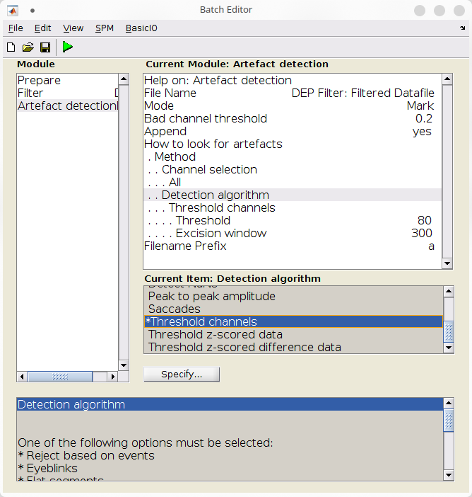
Add an “Artefact detection” batch (SPM >M/EEG >Preprocessing >Artefact detection),
Configure the batch to mark artefactual samples:
- Under file name, use the dependency button to refer to the file produced by the previous batch,
- Under “Mode”, select “Mark”,
- Under “Detection algorithm”, select “Threshold channels”,
- Under “Threshold”, specify “0.8”,
- Under “Excision window”, specify “300”,

Now that we have configured all the preprocessing steps, we can run the batch with the “Play” button.This batch should populate several files, the last being “afMdpil02.mat”, containing the data that we will model with convolution GLM.

S = [];

S.D                          = fullfile(workpath, D.fname);
S.mode                       = 'mark';
S.badchanthresh              = 0.2;
S.methods.channels           = {'all'};
S.methods.fun                = 'threshchan';
S.methods.settings.threshold = 80;
S.methods.settings.excwin    = 300;
S.append                     = 0;

D = spm_eeg_artefact(S);

prefix = ['a' prefix];

Finally, mark the channel ‘T8’ as bad:

D = spm_eeg_load(fullfile(workpath, [prefix name '.mat']));
D = D.badchannels(D.indchannel('T8'), 1);
save(D);

Constructing the convolution GLM model¶

Preliminary steps¶

We shall first load the file called “events.mat”. It contains the events onset times are stored in 3 cells corresponding to visual, auditory, and tactile events. Each cell contains the time in seconds (aligned to EEG data) at which the event occurs.

GUIScript

After loading the file in Matlab, go to the main SPM window and click on “Specify 1st-level” to start convolution modelling.

load(fullfile(datapath, 'events.mat'), 'events');
condnames = {'visual'; 'auditory'; 'tactile'};

We can then configure our convolution model.

Data, channels, timing¶

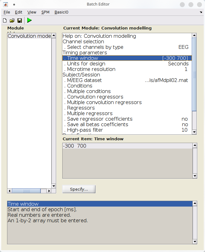
The first step is to tell SPM that we want to model the response on our EEG channels, in a peristimulus time window between 300ms before and 700ms after event onset.

GUIScript

Specify the channels to model under “Channel selection”:
- Remove the default entry (“Delete: All”)
- Click “Select channel by type” > “EEG”
Specify the timing parameters
- Under “Time window”, set \([-300 \;\; 700]\).
- Under “Unit for design”, set “seconds”
Under “M/EEG dataset”, select the last file produced at the previous section (“afMdpil02.mat”).

Setting the channels and timing parameters of the convolution model

convmodel = [];

convmodel.sess.D           = {fullfile(workpath, D.fname)};
convmodel.channels{1}.type = 'EEG';
convmodel.timing.timewin   = [-300 700];

Model structure¶

We can now specify the structure of the model, in particular, the timing of the events that we want to model.

For each condition (here, the sensory modalities), we need to specify the event times and duration, as well as other parameters such time or parametric modulation (SPM documentation on fMRI can be helpful in grasping these concepts). We use no parametric nor time modulation, and do not orthogonalize the basis set, which is already orthogonal.

Note that we want to model the response to instantaneous events (i.e. stick functions), whence we set the event duration to zero. However, under certain conditions one may want to use a specific duration, in which case the basis set will be convolved with a boxcar function.

GUIScript

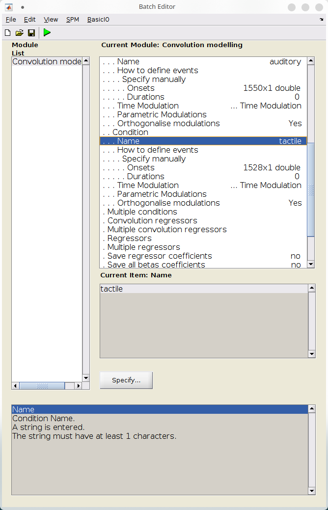
We will now specify the events for each condition. To do so:
- Click “Conditions” > “New: Condition”,
- Under name, set “visual”,
- We will set the event times manually. Under “How to define events”, select “Manually”
- Under “Onset”, type “events{1}”. This corresponds to the event onsets times from the “events.mat” file for event 1
- Under “Duration”, set 0. This will cause SPM to create stick functions at event onset.
- Leave over parameters of that section to their defaults
Repeat the previous steps for “auditory” and “tactile” events, whose onsets are stored in “events{2}” and “events{3}”.

Specifying the conditions of the convolution model

for c = 1:numel(condnames)
    % Condition name
    convmodel.sess.cond(c).name = condnames{c};

    % Event onset times in seconds, aligned to data
    convmodel.sess.cond(c).define.manual.onset = events{c};

    % Event duration in seconds, 0 for stick functions
    convmodel.sess.cond(c).define.manual.duration = 0;

    % Additional model parameters
    convmodel.sess.cond(c).tmod = 0;
    convmodel.sess.cond(c).pmod = struct('name', {}, 'param', {}, 'poly', {});
    convmodel.sess.cond(c).orth = 0;
end

Basis set¶

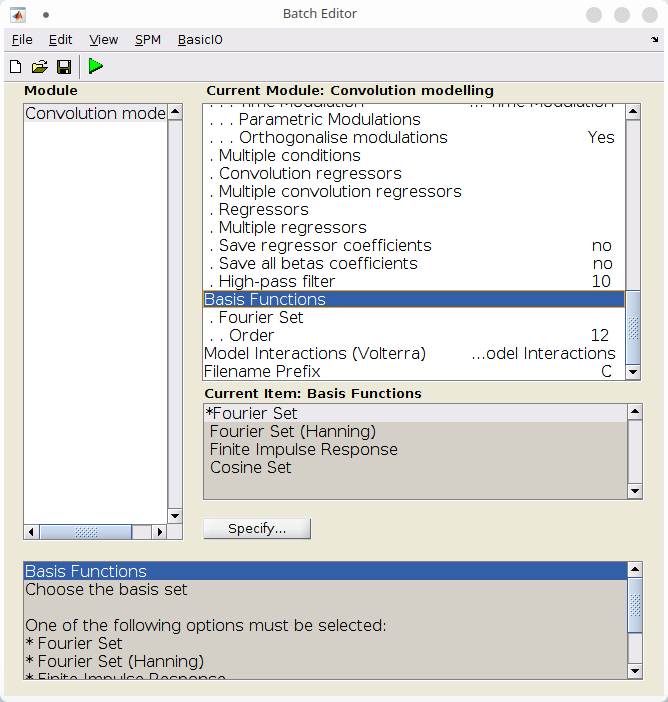
The last important step is to specify the basis set and its order.

Here, we use a Fourier basis set of order 12, which will consist of 12 pairs of sine and cosine at different frequencies, plus an intercept, for a total of 25 basis functions.

Basis set order and frequency resolution

Note that the order of the Fourier set interplays with the size of the time window: for a window of duration \(T\), the pairs of sine and cosine have frequencies \(1/T, 2/T, \dots, n/T\), where \(n\) is the order of the basis set. Thus, increasing the basis order will allow to capture faster and faster variations of the response (up to Nyquist frequency), at the expense of computational power. Here, we have a window of 1s and wlil be capturing changes in the response between 1 to 12Hz with a resolution of 1Hz.

GUIScript

Under “Basis Functions”:
- Make sure that the selected basis set is “Fourier Set”.
- Make sure that the “Order” is 12.

Setting the basis set of the convolution model — Specifying the conditions of the convolution model

convmodel.bases.fourier.order = 12;

Visualizing sample responses captured by a 12th order basis set

Let’s visualize the basis set and sample possible responses.

timevec = convmodel.timing.timewin(1):1000/D.fsample:convmodel.timing.timewin(2);

xBF        = struct;
xBF.dt     = 1/D.fsample;
xBF.name   = 'Fourier set';
xBF.length = diff(convmodel.timing.timewin)/1000;
xBF.order  = 12;

xBF = spm_get_bf(xBF);

weights   = randn(25, 4);
bfs       = xBF.bf;
responses = bfs * weights;

figure;
subplot(1, 2, 1);
plot(timevec, xBF.bf(:, 1:6), [0 0], [-1.5, 1.5], 'black');
xlim(convmodel.timing.timewin); ylim([-1.5, 1.5]);
subplot(1, 2, 2);
bounds = [min(responses, [], 'all')-1, max(responses, [], 'all')+1];
plot(timevec, responses, [0 0], bounds, 'black');
xlim(convmodel.timing.timewin); ylim(bounds);

Finals steps¶

GUIScript

A final step is to restablish the sensors type and locations using a Prepare batch (SPM > M/EEG > Preprocessing > Prepare).

Under “File name”, click “Dependency” and select the output from the Convolution modelling batch,
Under “Select task(s)”:
- Click “Set channel type”, and set “New channel type” to “EEG”
- Click “Project EEG sensors to 2D”.

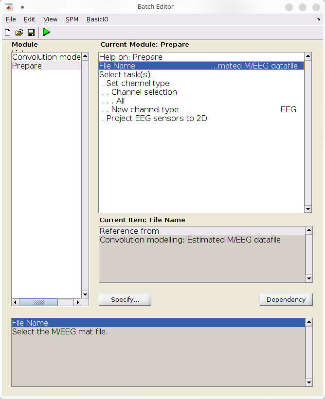
Final prepare batch to fix sensors types and locations.

Finally, run the batch with the “Play” button.

Set unused arguments to default

There are other more advanced parameters for this batch. We let them to default as we are not using them here. Interested users can look at the help for the “Convolution Modelling” batch in the GUI, and to that of the “fMRI Model Specification” batch (which is used under the hood).
```
convmodel.sess.hpf       = 10;
convmodel.sess.multi     = {''};
convmodel.timing.units   = 'secs';
convmodel.timing.utime   = 1;
convmodel.sess.multi_reg = {''};
convmodel.volt           = 1;
convmodel.sess.savereg   = 0;
convmodel.prefix         = 'C';
```

Put everything in a matlabbatch structure and run it

matlabbatch = {};
matlabbatch{1}.spm.meeg.modelling.convmodel = convmodel;

spm_jobman('run', matlabbatch);

prefix = ['C' prefix];

Restablish the 2D coordinates

coords = D.coor2D;
D      = spm_eeg_load(fullfile(workpath, [prefix name '.mat']));
D      = coor2D(D, 1:64, coords);
D      = chantype(D, ':', 'EEG');
save(D);

This produces a MEEG dataset with the deconvolved evoked responses for each of the three conditions.

Summary¶

To summarize, we have generated a Convolution GLM batch for our model to capture the response to each condition within a specific timeframe. Specifically, the design matrix created for this purpose has captured responses between 300ms before and 700ms after event onset, by expanding it on a 12th-order Fourier basis. This enables us to express the response as the weighted sum of 12 cosines and 12 sines, along with an intercept that captures the mean value. Note that the window of 1 second and the 12th-order Fourier basis allows us to capture oscillations between 1 and 12Hz, with a frequency resolution of 1Hz.

Using SPM, the convolution GLM generates a new M/EEG dataset that contains the deconvolved responses as evoked data.

Under the hood, SPM performs several operations…

It creates a design matrix \(X\) for our problem \(Y = X \beta + \varepsilon\), with time as rows and basis functions for each condition as columns.
It then inverts the model to obtain an estimate of the parameters that weight the basis set, represented by \(\beta = (X^TX)^{-1} X^T Y\). The rows of \(\beta\) correspond to the weight of each basis function, stacked for each condition \(c\).
It uses the basis function weights for condition \(c\) to construct the deconvolved responses, represented by \(y_c = x_{BF} \beta_c\).

Thus, the batch in this tutorial results in a M/EEG dataset of evoked responses, which contains three trials for each of our three conditions.

Results¶

Scalp maps¶

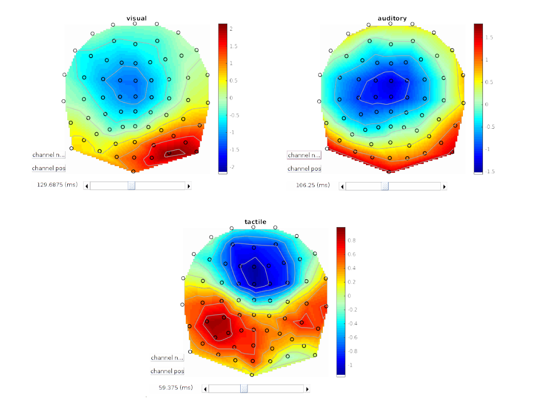
The results can be visualized in the SPM’s M/EEG viewer.

GUIScript

Click on the “Display…” menu in the main SPM window and select the data file “CafMdpil02.mat”.

spm_eeg_review(D);

Selecting EEG and then clicking on the scalp image shows the deconvolved response over the scalp. By positioning the peristimulus time cursor tenth to hundreds of milliseconds after stimulus onset, we can observe the stereo-typical scalp maps of visual, auditory, and tactile stimuli (Figure 1.8).

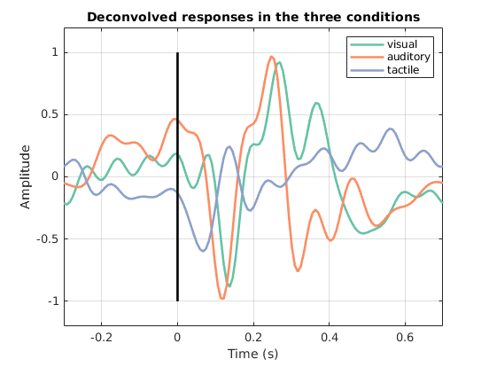
Scalp maps of deconvolved responses to the different stimuli at particular time of interest.

Average response over frontocentral channels.¶

We look at the average response on the fronto-central channels in the 3 different conditions, to see how different are the deconvolved responses.

GUIScript

Copy and past the following code in Matlab command window, or in a new script. Make sure that you are in the same directory as the file “CafMdpil02.mat”.

D  = spm_eeg_load('CafMdpil02.mat'); 
Ic = D.indchannel({ ...
    'Fz', 'F1', 'F2', 'F3', 'F4'...
    'FCz', 'FC1', 'FC2', 'FC3', 'FC4'...
    'Cz', 'C1', 'C2', 'C3', 'C4'...
});
y = squeeze(mean(D(Ic, :, :), 1));
t = D.time();

figure; hold on;
plot(t, y, 'LineWidth', 2);
plot([0 0], [-1 1], 'k', 'LineWidth', 2);
legend(D.condlist); box on; grid on;
xlim([min(t), max(t)]); ylim([-1.2 1.2]);
xlabel('Time (s)'); ylabel('Amplitude');
title('Deconvolved responses in the three conditions');
hold off;

Ic = D.indchannel({ ...
    'Fz', 'F1', 'F2', 'F3', 'F4'...
    'FCz', 'FC1', 'FC2', 'FC3', 'FC4'...
    'Cz', 'C1', 'C2', 'C3', 'C4'...
});
y = squeeze(mean(D(Ic, :, :), 1));
t = D.time();

figure; hold on;
plot(t, y, 'LineWidth', 2);
plot([0 0], [-1 1], 'k', 'LineWidth',2);
legend(D.condlist); box on; grid on;
xlim([min(t), max(t)]); ylim([-1.2 1.2]);
xlabel('Time (s)'); ylabel('Amplitude');
title('Deconvolved responses in the three conditions');
hold off;

Average responses over fronto-central channels for the different stimuli.

Concluding remarks¶

In summary, convolution modelling proves to be a powerful tool to disentangle responses that overlap over time (Figure 1.9), and can be used as a preliminary step to extract event related responses for subsequent statistical analysis.

In practice, convolution modelling can replace the classical “epoching and averaging” steps of an evoked response pipeline. As such, it produces an evoked response dataset that can be used in second-level analysis.

Acknowledgements¶

We thank Bernhard Spitzer for putting up the code from which this tutorial derives and for kindly allowing us to share the data analysed in this chapter.

V. Litvak, Ashwani Jha, G. Flandin, and K.J. Friston. Convolution models for induced electromagnetic responses. NeuroImage, 64():388–398, 2013. doi:10.1016/j.neuroimage.2012.09.014. ↩
Bernhard Spitzer, Felix Blankenburg, and Christopher Summerfield. Rhythmic gain control during supramodal integration of approximate number. NeuroImage, 129:470–479, 2016. ↩