MEG analysis 
Preprocessing the MEG data
First change directory to the MEG subdirectory (either in MATLAB, or via the “CD” option in the SPM “Utils” menu)
Adjust trigger latency
For the EEG data, the faces were displayed directly via a CRT monitor. For the MEG data on the other hand, the faces were displayed inside the MSR via a projector. This projector produces a delay of 1.5 screen refreshes, which at 60Hz, is 25ms. This means that the subject actually saw the stimuli 25ms after the trigger was sent to the MEG acquisition machine. To correct for this visual delay, we will illustrate how to manipulate “trial” structures1. First, we need to read in the triggers from the MEG data (unlike the EEG dataset, the MEG dataset contains information about trial type so we can define the correct condition labels already at this stage). To do this, type the following in the MATLAB window:
[trl, conditionlabels, S] = spm_eeg_definetrial;
and follow these steps:
-
Select the
SPM_CTF_MEG_example_faces1_3D.ds/SPM_CTF_MEG_example_faces1_3D.meg4file. -
Enter
-200for “Start of trial in PST [ms]” and600to “End of trial in PST [ms]“. -
Enter 2 for “How many conditions?”.
-
Enter “
faces” for “Label of condition 1”. A dialog with a list of events will come up and Select the event with typeUPPT001_upand Value 1. -
Enter “
scrambled” for “Label of condition 2”. Select the even with typeUPPT001_upand Value 2. -
Answer “no” to the question about reviewing trials.
-
Answer “yes” to the prompt to save the trial definition.
-
Enter a filename like
trials_run1.matand save in the MEG directory.
Then type load trials_run1.mat in MATLAB, to see the contents of the
file you just saved. It contains two variables, trl and
conditionlabels. The trl variable contains as many rows as triggers
were found (across all conditions) and three columns: the initial sample
of the epoch, the final sample of the epoch and the offset in samples
corresponding to a peristimulus time of 0. The sampling rate for the MEG
data was 480Hz (as can be found in the S.fsample field of the
structure S returned by the spm_eeg_definetrial call above). Thus
the figure of -96 samples in the third column corresponds to the 200ms
baseline period that you specified. Now we need to shift the initial and
final samples of the epochs by 25ms. You can do this by typing:
    trl(:,1:2) = trl(:,1:2) + round(25*S.fsample/1000);
    save trials_run1 trl conditionlabels
The new trial definition is thus resaved, and we can use this file when next converting the data.
Convert
Press the Convert button, and in the file
selection window again select the SPM_CTF_MEG_example_faces1_3D.ds
subdirectory and the SPM_CTF_MEG_example_faces1_3D.meg4 file. At the
prompt “Define settings?” select “yes”. Here we will use the option to
define more precisely the part of data that should be read during
conversion. Answer “trials” to “How to read?”, and “file” to “Where to
look for trials?”. Then in the file selector window, select the new
trials_run1.mat file. Press “no” to “Read across trials?” and select
“meg” for “What channels?”. Press “no” to avoid saving the channel
selection. Press “Enter” to accept the default suggestion for the name
of the output dataset. Two files will be generated
espm8_SPM_CTF_MEG_example_faces1_3D.mat and
espm8_SPM_CTF_MEG_example_faces1_3D.dat. After the conversion is
complete the data file will be automatically opened in the SPM8
reviewing tool. If you click on the “MEG” tab you will see the MEG data
which is already epoched. By pressing the “intensity rescaling” button
(with arrows pointing up and down) several times you will start seeing
MEG activity.
Baseline correction
We need to perform baseline correction as it is not done automatically
during conversion. This will prevent excessive edge artefacts from
appearing after subsequent filtering and downsampling. Select
Baseline correction from the “Other”
drop-down menu and select the espm8_SPM_CTF_MEG_example_faces1_3D.mat
file. Enter \([-200\: 0]\) for “Start and stop of baseline [ms]“. The
progress bar will appear and the resulting data will be saved to dataset
bespm8_SPM_CTF_MEG_example_faces1_3D.{mat,dat}.
Downsample
Select Downsample from the “Other”
drop-down menu and select the bespm8_SPM_CTF_MEG_example_faces1_3D.mat
file. Choose a new sampling rate of 200 (Hz). The progress bar will
appear and the resulting data will be saved to dataset
dbespm8_SPM_CTF_MEG_example_faces1_3D.{mat,dat}.
Batch preprocessing
Here we will preprocess the second half of the MEG data using using the SPM8 batch facility to demonstrate this third (after interactive GUI and Matlab script) possibility. First though, we have to correct the visual onset latency for the second run, repeating the above steps that you did for the first run:
[trl, conditionlabels, S] = spm_eeg_definetrial;
and select the SPM_CTF_MEG_example_faces2_3D.ds subdirectory and the
SPM_CTF_MEG_example_faces2_3D.meg4 file. Then enter -200 for “Start
of trial in PST [ms]” and 600 to “End of trial in PST [ms]“. Enter
2 for “How many conditions?”. Enter “faces” for “Label of condition
1”. A dialog with a list of events will come up. Select the event with
type “UPPT001_up” and Value 1. Enter scrambled for “Label of
condition 2”. Select the event with type “UPPT001_up” and Value 2.
Answer “no” to the question about reviewing trials, but “yes” to the
prompt to save the trial definition. Enter a filename like
trials_run2.mat and save in the MEG directory. Then type:
    load trials_run2
    trl(:,1:2) = trl(:,1:2)+round(25*S.fsample/1000);
    save trials_run2 trl conditionlabels
Now press the Batch button (lower right
corner of the SPM8 menu window). The batch tool window will appear. We
will define exactly the same settings as we have just done using the
interactive GUI. From the “SPM” menu, “M/EEG” submenu select “M/EEG
Conversion”. Click on “File name” and select the
SPM_CTF_MEG_example_faces2_3D.meg4 file from
SPM_CTF_MEG_example_faces2_3D.ds subdirectory. Click on “Reading mode”
and switch to “Epoched”. Click on “Epoched” and choose “Trial file”,
double-click on the new “Trial file” branch and then select the
trials_run2.mat file. Then click on “Channel selection” and select MEG
from the menu below. Finally enter espm8_SPM_CTF_MEG_example_faces2_3D
for “Output filename” to be consistent with the file preprocessed
interactively.
Now select “M/EEG Baseline correction” from the “SPM” menu, “M/EEG”
submenu. Another line will appear in the Module list on the left. Click
on it. The baseline correction configuration branch will appear. Select
“File name” with a single click. The file that we need to downsample has
not been generated yet but we can use the “Dependency” button. A dialog
will appear with a list of previous steps (in this case just the
conversion) and we can set the output of one of these steps as the input
to the present step. Now just enter enter \(-200\: 0\) for “Baseline”.
Similarly we can now add “M/EEG Downsampling” to the module list, define
the output of baseline correction step for “File name” and 200 for the
“New sampling rate”. This completes our batch. We can now save it for
future use (e.g, as batch_meg_preprocess and run it by pressing the
green “Run” button. This will generate all the intermediate datasets and
finally dbespm8_SPM_CTF_MEG_example_faces2_3D.{mat,dat}.
Merge
We will now merge the two epoched files we have generated until now and
continue working on the merged file. Select the
Merge command from the “Other” drop-down
menu. In the selection window that comes up click on
dbespm8_SPM_CTF_MEG_example_faces1_3D.mat and
dbespm8_SPM_CTF_MEG_example_faces2_3D.mat. Press “done”. Answer “Leave
as they are” to “What to do with condition labels?”. A new dataset will
be generated called cdbespm8_SPM_CTF_MEG_example_faces1_3D.{mat,dat}.
Reading and preprocessing data using Fieldtrip
Yet another even more flexible way to pre-process data in SPM8 is to use
the Fieldtrip toolbox (http://www.ru.nl/neuroimaging/fieldtrip/) that
is distributed with SPM. All the pre-processing steps we have done until
now can also be done in Fieldtrip and the result can then be converted
to SPM8 dataset. An example script for doing so can be found in the
man\(\backslash\)example_scripts\(\backslash\)spm_ft_multimodal_preprocessing.m.
The script will generate a merged dataset and save it under the name
ft_SPM_CTF_MEG_example_faces1_3D.{mat,dat}. The rest of the analysis
can then be done as below. This option is more suitable for expert users
well familiar with Matlab. Note that in the script ft_ prefix is added
to the names of all Fieldtrip functions. This is a way specific to SPM8
to call the functions from Fieldtrip version included in SPM
distribution and located under external\(\backslash\)fieldtrip.
Prepare
In this section we will add the separately measured headshape points to
our merged dataset. This is useful when one wants to improve the
coregistration using head shape measured outside the MEG. Also in some
cases the anatomical landmarks detectable on the MRI scan and actual
locations of MEG locator coils do not coincide and need to be measured
in one common coordinate system by an external digitizer (though this is
not the case here). First let’s examine the contents of the headshape
file. If you load it into MATLAB workspace (type load headshape.mat),
you will see that it contains one MATLAB structure called shape with
the following fields:
-
.unit- units of the measurement (optional) -
.pnt- Nx3 matrix of headshape points -
.fid- substruct with the fields .pnt - Kx3 matrix of points and .label -Kx1 cell array of point labels.
The difference between shape.pnt and shape.fid.pnt is that the
former contains unnamed points (such as continuous headshape
measurement) whereas the latter contains labeled points (such as
fiducials). Note that this Polhemus space (which will define the “head
space”) has the X and Y axes switched relative to MNI space.
Now select Prepare from the “Other” menu
and in the file selection window select
cdbespm8_SPM_CTF_MEG_example_faces1_3D.mat. A menu will appear at the
top of SPM interactive window (bottom left window). In the “Sensors”
submenu choose “Load MEG Fiducials/Headshape”. In the file selection
window choose the headshape.mat file and save the dataset with
File/Save.
If you do not have a separately measured headshape and are planning to use the original MEG fiducials for coregistration, this step is not necessary. As an exercise, you can skip it for the tutorial dataset and later do the coregistration without the headshape and see if it affects the results.
Basic ERFs
Press the Averaging button and select the
cdbespm8_SPM_CTF_MEG_example_faces1_3D.mat file. Answer “yes” to “Use
robust averaging?”. You can either save the weights if you want to
examine them or not save if you want the averaging to work faster since
the weights dataset that needs to be written is quite large. Answer “no”
to “weight by condition” and accept the default “Offset of the weighting
function”. A new dataset will be created in the MEG directory called
mcdbespm8_SPM_CTF_MEG_example_faces1_3D.{mat,dat} (“m” for “mean”).
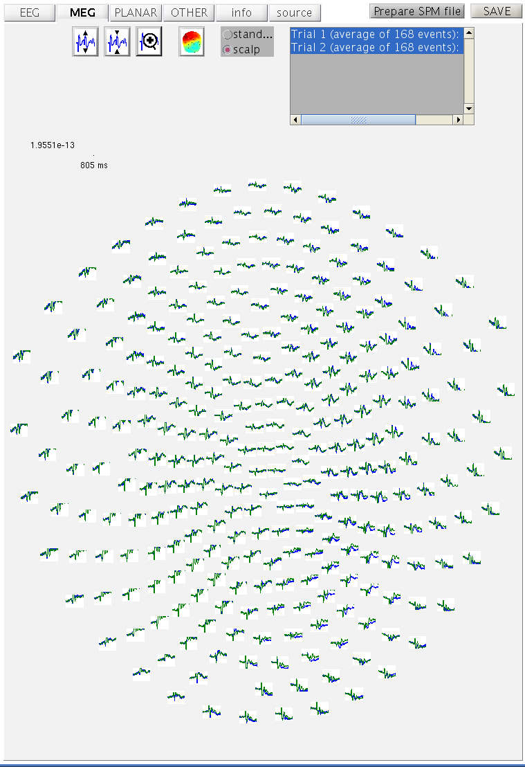
As before, you can display these data by “Display: M/EEG” and selecting
the mcdbespm8_SPM_CTF_MEG_example_faces1_3D.mat. In the MEG tag with
the scalp radio button selected, hold the Shift key and select
trial-type 2 with the mouse in the bottom right of the window to see
both conditions superimposed (as
Figure 1).
mcdbespm8_SPM_CTF_MEG_example_faces1_3D.mat) for all 275
MEG channels. Select “Contrast” from the “Other” pulldown menu on the SPM window. This
function creates linear contrasts of ERPs/ERFs. Select the
mcdbespm8_SPM_CTF_MEG_example_faces1_3D.mat file, enter \([1\: -1]\) as
the first contrast and label it “Difference”, answer “yes” to “Add
another”, enter \([1/2\: 1/2]\) as the second contrast and label it
“Mean”. Press “no” to the question “Add another” and not to “weight by
num replications”. This will create new file
wmcdbespm8_SPM_CTF_MEG_example_faces1_3D.mat, in which the first
trial-type is now the differential ERF between faces and scrambled
faces, and the second trial-type is the average ERF for faces and
scambled faces.
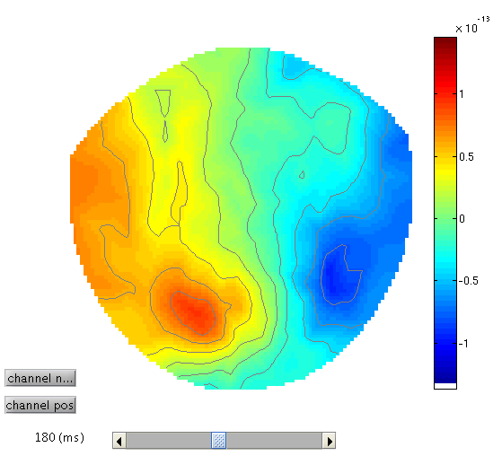
To see the topography of the differential ERF, select “Display: M/EEG”, MEG tab and click on Trial 1, press the “topography” button at the top of the window and scroll to 180ms for the latency to produce Figure 2.
You can move the slider left and right to see the development of the M170 over time.
Time-Frequency Analysis
SPM can use several methods for time-frequency decomposition. We will use Morlet wavelets for our analyses.
Select the time-frequency option under
the “Other” pull-down menu. SPM batch tool with time-frequency
configuration options will appear. Double-click on “File name” and
select the cdbespm8_SPM_CTF_MEG_example_faces1_3D.mat file. Then click
on “Channel selection” and in the box below click on “Delete: All(1)”
and then on “New: Custom channel”. Double-click on “Custom channel” and
enter “MLT34”.2 Double-click on “Frequencies of interest” and type
[5:40] (Hz). Click on “Spectral estimation” and select “Morlet wavelet
transform”. Change the number of wavelet cycles from 7 to 5. This factor
effectively trades off frequency vs time resolution, with a lower order
giving higher temporal resolution. Select “yes” for “Save phase?”.
This will produce two new datasets,
tf_cdbespm8_SPM_CTF_MEG_example_faces1_3D.{mat,dat} and
tph_cdbespm8_SPM_CTF_MEG_example_faces1_3D.{mat,dat}. The former
contains the power at each frequency, time and channel; the latter
contains the corresponding phase angles.
Here we will not baseline correct the time-frequency data because for frequencies as low as 5Hz, one would need a longer pre-stimulus baseline, to avoid edge-effects3. Later, we will compare two trial-types directly, and hence any pre-stimulus differences will become apparent.
Press the Averaging button and select the
tf_cdbespm8_SPM_CTF_MEG_example_faces1_3D.mat file. You can use
straight (or robust if you prefer) averaging to compute the average
time-frequency representation. A new file will be created in the MEG
directory called mtf_cdbespm8_SPM_CTF_MEG_example_faces1_3D.{mat,dat}.
Note that you can use the reviewing tool to review the time-frequency
datasets.
This contains the power spectrum averaged over all trials, and will
include both “evoked” and “induced” power. Induced power is
(high-frequency) power that is not phase-locked to the stimulus onset,
which is therefore removed when averaging the amplitude of responses
across trials (i.e, would be absent from a time-frequency analysis of
the mcdbespm8_SPM_CTF_MEG_example_faces1_3D.mat file).
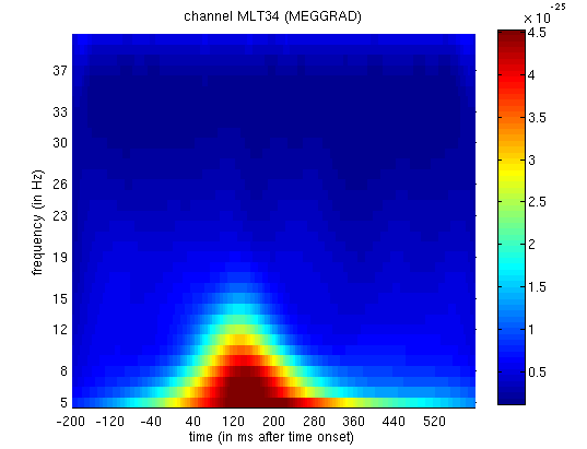
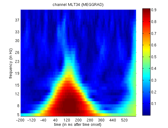
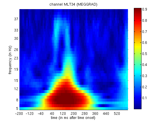
The power spectra for each trial-type can be displayed using the usual
Display button and selecting the
mtf_cdbespm8_SPM_CTF_MEG_example_faces1_3D.mat file. This will produce
a plot of power as a function of frequency (y-axis) and time (x-axis)
for Channel MLT34. If you use the “trial” slider to switch between
trial(types) 1 and 2, you will see the greater power around 150ms and
10Hz for faces than scrambled faces (click on the magnifying glass icon
and on the single channel to get scales for the axes, as in
Figure 3). This corresponds to the M170
again.
We can also look at evidence of phase-locking of ongoing oscillatory activity by averaging the phase angle information. We compute the vector mean (by converting the angles to vectors in Argand space), which yields complex numbers. We can generate two kinds of images from these numbers. The first is an image of the angles, which shows the mean phase of the oscillation (relative to the trial onset) at each time point. The second is an image of the absolute values (also called “Phase-Locking Value”, PLV) which lie between 0 for no phase-locking across trials and 1 for perfect phase-locking.
Press the Averaging button and select the
tph_cdbespm8_SPM_CTF_MEG_example_faces1_3D.mat file. This time you
will be prompted for either “angle” or “abs(PLV)” average, for which you
should select “abs(PLV)”. The MATLAB window will echo:
  mtph_cdbespm8_SPM_CTF_MEG_example_faces1_3D.mat: Number of replications per contrast:
  average faces: 168 trials, average scrambled: 168 trials
and a new file will be created in the MEG directory called
mtph_cdbespm8_SPM_CTF_MEG_example_faces1_3D.mat.
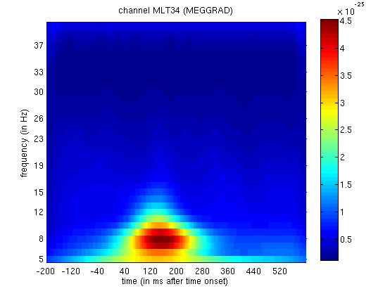
If you now display the file
mtph_cdbespm8_SPM_CTF_MEG_example_faces1_3D.mat file, you will see PLV
as a function of frequency (y-axis) and time (x-axis) for Channel MLT34.
Again, if you use the “trial” slider to switch between trial(types) 1
and 2, you will see greater phase-locking around for faces than
scrambled faces at lower frequencies, as in
Figure 4. Together with the above power
analysis, these data suggest that the M170 includes an increase both in
power and in phase-locking of ongoing oscillatory activity in the alpha
range (Henson et al, 2005b).
2D Time-Frequency SPMs
Analogous to Section [multimodal:eeg:3DSPM], we can also use Random Field Theory to correct for multiple statistical comparisons across the 2-dimensional time-frequency space.
Select Convert to images in the “Other”
pulldown menu, and select the
tf_cdbespm8_SPM_CTF_MEG_example_faces1_3D.mat file. Usually you would
be asked whether you want to average over channels or frequencies. In
this case there is only one channel in this dataset, so the “channels”
option will be selected automatically.
This will create 2D time-frequency images for each trial of the two
types with dimensions \(36\times 161\times 1\), as for the example shown
in Figure 5. These images can be found in
the subdirectories 1ROI_TF_trialtype_faces and
1ROI_TF_trialtype_scrambled of the new directory created
tf_cdbespm8_SPM_CTF_MEG_example_faces1_3D, and examined by pressing
“Display: images” on the main SPM window.
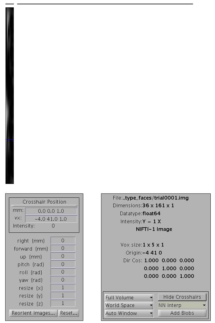
1ROI_TF_trialtype_faces subdirectory. The bottom left
section is through frequency (x) and time (y) (the other images are
strips because there is only one value in the z dimension, i.e, this is
really a 2D image).As in Section [multimodal:eeg:3Dsmooth], these images can be further smoothed in time and frequency if desired.
Then as in Section [multimodal:eeg:3DSPM], we then take these images into an unpaired t-test across trials to compare faces versus scrambled faces. We can then use classical SPM to identify times and frequencies in which a reliable difference occurs, correcting across the multiple comparisons entailed (Kilner et al, 2005).
First create a new directory, eg. mkdir TFstatsPow.
Then press the specify 2nd level button,
select “two-sample t-test” (unpaired t-test), and define the images for
“group 1” as all those in the subdirectory trialtype_faces (using
right click, and “select all”) and the images for “group 2” as all those
in the subdirectory trialtype_scrambled. Finally, specify the new
TFstatsPow directory as the output directory. (Note that this will be
faster if you saved and could load an SPM job file from
Section [multimodal:eeg:3DSPM] in
order to just change the input files and output directory.) Then add an
“Estimate” module from the “SPM” tab, and select the output from the
previous factorial design specification stage as the dependency input.
Press “Run” (green arrow button).
Press Results and define a new T-contrast as \([1\: -1]\). Keep the default contrast options, but threshold at \(p<.05\) FWE corrected for the whole search volume, and then select “Time-Frequency” for the “Data Type”. Then press “whole brain”, and the Graphics window should now look like that in Figure 6.
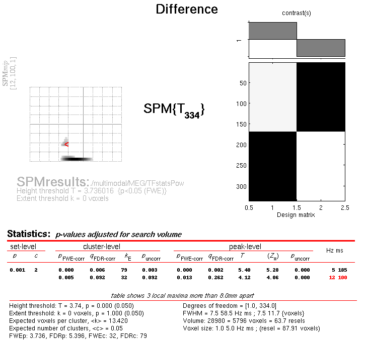
This will list two “regions” within the 2D time-frequency space in which faces produce greater power than scrambled faces, having corrected for multiple T-tests across pixels. The larger one has a maximum at 5 Hz and 185 ms post-stimulus, corresponding to the M170 seen earlier in the averaged files (but now with a statistical test of its significance, in terms of evoked and induced power). The second, smaller region has a maximum at 12 Hz and 100 ms, possibly corresponding to a smaller but earlier effect on the M100 (also sometimes reported, depending on what faces are contrasted with).
“Imaging” reconstruction of total power for each condition 
In Section [multimodal:eeg:3D] we localised the differential evoked potential difference in EEG data corresponding to the N170. Here we will localise the total power of faces, and of scrambled faces, ie including potential induced components (see Friston et al, 2006).
Press the “3D source reconstruction” button, and press the “load” button
at the top of the new window. Select the
cdbespm8_SPM_CTF_MEG_example_faces1_3D.mat file and type a label (eg
M170) for this analysis.
Press the “MRI” button, select the smri.img file within the sMRI
sub-directory and select the “normal” mesh.
If you have not used this MRI image for source reconstruction before,
this step will take some time while the MRI is segmented and the
deformation parameters computed (see
Section [multimodal:eeg:3D] for more
details on these files). When meshing has finished, the cortex (blue),
inner skull (red) and scalp (orange) meshes will also be shown in the
Graphics window with slices from the sMRI image. This makes it possible
to verify that the meshes indeed fit the original image well. The field
D.inv{1}.mesh will be updated. Press “save” in top right of window to
update the corresponding mat file on disk.
Both the cortical mesh and the skull and scalp meshes are not created directly from the segmented MRI, but rather are determined from template meshes in MNI space via inverse spatial normalisation (Mattout et al, 2007; Henson et al, 2009a).
Press the “Co-register” button. You will be asked for each of the 3
fiducial points to specify its location on the MRI images. This can be
done by selecting a corresponding point from a hard-coded list
(“select”). These points are inverse transformed for each individual
image using the same deformation field that is used to create the
meshes. The other two options are typing the MNI coordinates for each
point (“type”) or clicking on the corresponding point in the image
(“click”). Here, we will type coordinates based on where the
experimenter defined the fiducials on the smri.img. These coordinates
can be found in the smri_fid.txt file also provided. So press “type”
and for “nas”, enter [0 91 -28]; for “lpa” press “type” and enter
[-72 4 -59]; for “rpa” press “type” and enter [71 -6 -62]. Finally,
answer “no” to “Use headshape points?” (see EEG
Section [multimodal:eeg:3D]).
This stage coregisters the MEG sensor positions with the structural MRI
and cortical mesh, via an approximate matching of the fiducials in the
two spaces, followed by a more accurate surface-matching routine that
fits the head-shape function (measured by Polhemus) to the scalp that
was created in the previous meshing stage via segmentation of the MRI.
When coregistration has finished, the field D.inv{1}.datareg will be
updated. Press “save” in top right of window to update the corresponding
mat file on disk. With the MATLAB Rotation tool on (from the “Tools” tab
in the SPM Graphics window, if not already on), right click near the top
image and select “Go to X-Z” view. This should produce a figure like
that in Figure 7, which you can rotate with the
mouse to check all sensors. Note that the data are in head space (not
MNI space), in this case corresponding to the Polhemus space in which
the X and Y dimensions are swapped relative to MNI space.
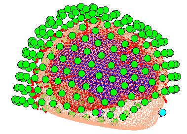
Press the “Forward Model” button. Choose “MEG Local Spheres” (you may also try the other options; see Henson et al, 2009a). A figure will be displaying showing the local (overlapping) spheres fit to each sensor, and final the set of all spheres.
Press “Invert”, select “Imaging”, select “yes” to “All conditions or trials?”, and “Standard” for the model (i.e, to use defaults; you can customise a number of options if you press Custom instead) (see Friston et al, 2008, for more details about these parameters). There will be lead field computation followed by the actual inversion. A summary plot of the results will be displayed at the end.
You can now explore the results via the 3D reconstruction window. If you type 180 into the box in the bottom right (corresponding to the time in ms) and press “mip”, you should see several ventral temporal hotspots, as in Figure 8. Note that this localisation is different from the previous EEG localisation because 1) condition 1 now refers to faces, not the difference between faces and scrambled faces, and 2) the results reflect total power (across trials), induced and evoked, rather than purely evoked4. The timecourses come from the peak voxel (with little evidence of a face/scrambled difference for this particular maximum). The red curve shows the condition currently being shown (corresponding to the “Condition 1” toggle bar in the reconstruction window); the grey curve(s) will show all other conditions. If you press the "condition 1" toggle, it will change to Condition 2, which is the total power for scrambled faces, then press “mip” again and the display will update (note the colours of the lines have now reversed from before, with red now corresponding to scrambled faces).
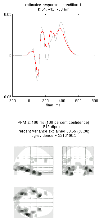
If press “movie”, you will see the changes in the source strengths over peristimulus time (from the limits 0 to 300ms currently chosen by default).
If you press “render” it will open a graphical interface that is very useful to explore the data (the buttons are fairly self-explanatory).
You can also explore the other inversion options, like COH and IID, which you will note give more superficial solutions (a known problem with standard minimum norm; see also Friston et al, 2008; Henson et al, 2009a). To do this quickly (without repeating the MRI segmentation, coregistration and forward modelling), press the “new” button in the reconstruction window, which by default will copy these parts from the previous reconstruction.
In the following we will concentrate on how one prepares this single subject data for subsequent entry into a group analysis.
Press the “Window” button in the reconstruction window, enter “150 200” as the timewindow of interest and “5 15” as the frequency band of interest (from the SPM time-frequency analysis, at least from one channel). Then choose the “induced” option. After a delay (as SPM calculates the power across all trials) the Graphics window will show the mean activity for this time/frequency contrast (for faces alone, assuming the condition toggle is showing “condition 1”).
If you then press “Image”, SPM will write 3D NIfTI images corresponding to the above contrast for each condition:
    cdbespm8_SPM_CTF_MEG_example_faces1_3D_1_t150_200_f5_15_1.nii
    cdbespm8_SPM_CTF_MEG_example_faces1_3D_1_t150_200_f5_15_2.nii
The last number in the file name refers to the condition number; the
number following the dataset name refers to the reconstruction number
(i.e. the number in red in the reconstruction window, i.e, D.val, here
1).
The smoothed results for Condition 1 will also be displayed in the Graphics window, together with the normalised structural. Note that the solution image is in MNI (normalised) space, because the use of a canonical mesh provides us with a mapping between the cortex mesh in native space and the corresponding MNI space.
You can also of course view the image with the normal SPM “Display:image” option, and locate the coordinates of the “hotspots” in MNI space. Note that these images contain RMS (unsigned) source estimates (see Henson et al, 2007).
If you want to see where activity (in this time/freq contrast) is
greater for faces and scrambled faces, you can use SPM ImCalc facility
to create a difference image of
cdbespm8_SPM_CTF_MEG_example_faces1_3D__t150__f5__1.nii -
cdbespm8_SPM_CTF_MEG_example_faces1_3D__t150__f5__2.nii: you should
see bilateral fusiform. For further discussion of localising a
differential effect (as in
Section [multimodal:eeg:3D] with ERPs),
vs taking the difference of two localisations, as here, see Henson et al
(2007). The above images can then be used at the second level (assuming
one also has data from other subjects) to look for effects that are
consistent over a group of subjects.
-
Alternatively, you could correct by 1 refresh, to match the delay in the EEG data. ↩
-
You can of course obtain time-frequency plots for every channel, but it will take much longer (and result in a large file). ↩
-
For example, for 5Hz, one would need at least N/2 x 1000ms/5, where N is the order of the Morlet wavelets (i.e, number of cycles per Gaussian window), e.g, 600ms for a 6th-order wavelet. ↩
-
Though in reality, most of the power is low-frequency and evoked ↩