One-sample t-test
In this this tutorial we will perform a one-sample t-test at each voxel in the brain. This will tell us if and where in the brain our group responds to a specific task condition or experimental contrast on average.
Here we will check if there is an overall effect of the task (i.e. contrast con_0009.nii - for a reminder of first-level contrasts, check the previous page).
Specifying the model
- Navigate to
derivatives/second_leveland make a folder for this analysis. Make an empty folder where you will save your results. Name it something meaningful to you, e.g.one_sample_ttest_task. - Select
Specify 2nd levelfrom the SPM menu. - In the pop-up batch editor window, select your newly created output folder (directory) by clicking
Directoryand navigating toderivatives/second_level/one_sample_ttest_taskin the selection box. - Define your statistical model by selecting
DesignOne-sample t-test(this is selected by default). - Select
ScansSpecify.... - Now, using the selection window recursively filter for contrast
con_0009.nii. To do this, navigate toderivatives/first-levelvia the left-hand side panel. In the filter box, type in^con_0009.niiand click theRecbutton. You should see 40 volumes selected in the bottom window. Double check that the correct contrast and subjects have been selected. Confirm selection by pressingDone. - Optional: You can also include covariates and/or nuisance variables in your model. These can be specified under
CovariatesandMultiple covariates. Your covariates should be formatted as columns with rows corresponding to each participant. Always make sure the order in which you input your partipant’s contrasts in the previous step is the same as the order in your covariates list. - From the drop-down menu panel, select
SPMStatsModel estimation. - Navigate to
Model estimationin the left-hand panel of the batch window. - Press
Select SPM.matDependencyFactorial design specification: SPM.mat fileOK. - From the drop-down menu panel, select
SPMStatsContrast manager. - Within the
Contrast manager, click onSelect SPM.matDependencyModel estimation: SPM.mat fileOK. - You can now start specifying your contrasts of interest in
Contrast sessions. We’ll include two t-contrasts, one looking at activations and one looking at deactivations. SelectContrast sessionsNew: T-contrast. - Give your contrast an informative name,
NameSpecify.... We’ll name this contrastactivations. - Specify your contrast weight,
Weights vectorSpecify...1. -
Now click on Contrast Sessions and add another
T-contrastcalling itdeactivationsand giving it a weight of-1.F-contrasts
You can also specify an
F-contrastwith a contrast weight of1to look at both activations and deactivations within one contrast. -
Optional: You can also add contrasts exploring the effects of your covariates by specifying contrast weights for the corresponding columns of the design matrix.
- When you’re ready, save your batch and press to run your analysis.
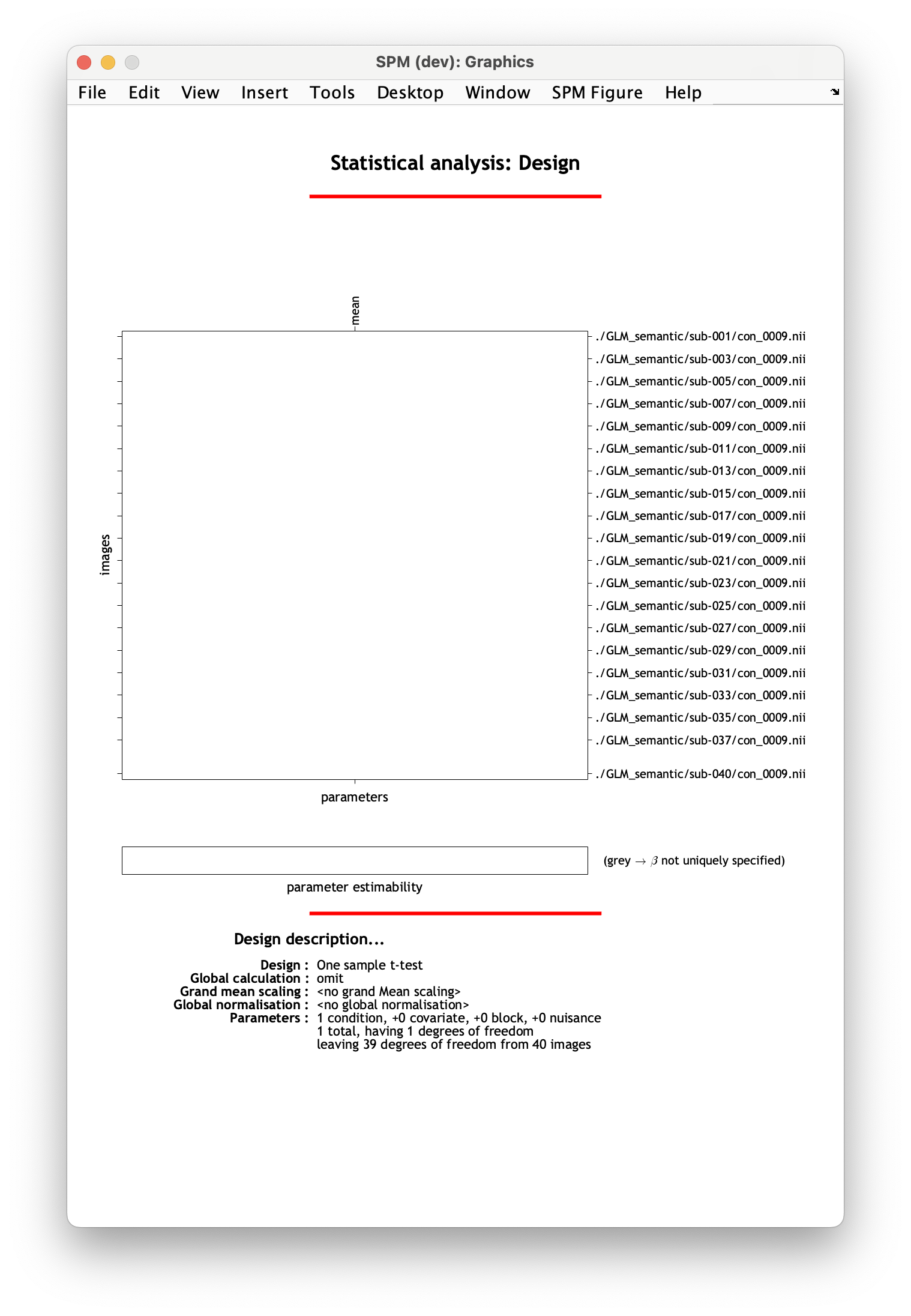
Unless you have specified additional covariates, the design matrix for your model should have one column denoting the group effect and look like this:
Viewing the results
To view the results of your analysis, return to the main SPM window and select Results, then select the SPM.mat file corresponding to your analysis. In our case, this will be in derivatives/second_level/one_sample_ttest_task. Choose a contrast to view, e.g. positive.
SPM will now let you select masking and multiple comparisons correction. Select the following in the SPM window:
Apply maskingnoneP-value adjustment to controlFWEP-value0.05Extent threshold (voxels)0
A bit more about SPM results options
Apply masking- this option allows you examine your results within a specific region, specified either from a contrast, predefined image, or atlas. To interrogate all voxels in the brain, selectnone.P-value adjustment to control- this lets you select whether you want to display the results as uncorrected for multiple comparisons(none) or with a FWE voxel/peak-level correction (FWE).P-value- here you can specify your p-threshold.Extent threshold (voxels)- this allows you set a threshold of the minimum number of contiguous voxels in a cluster to be displayed. This can be used in cluster correction.
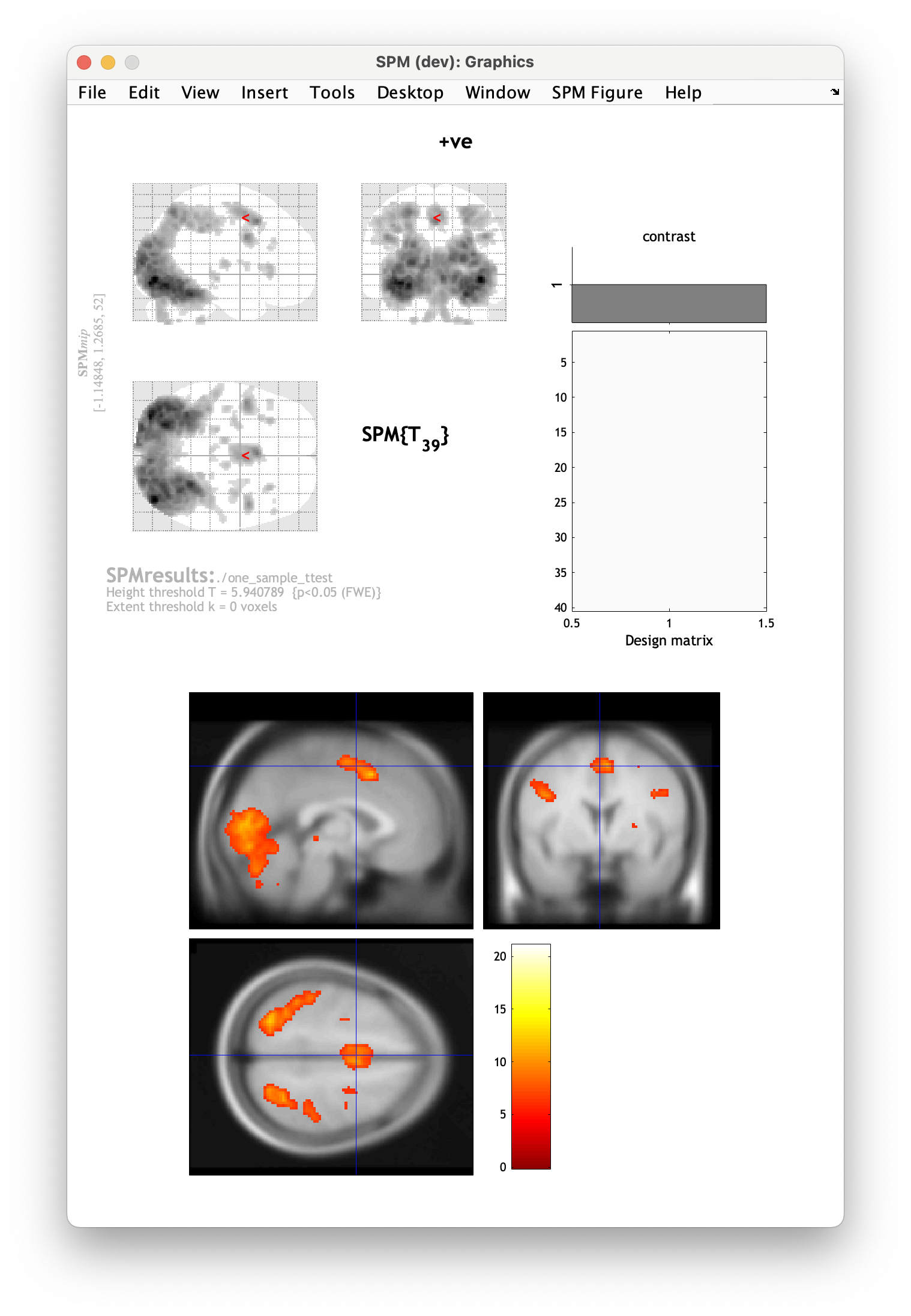
After going through these steps, SPM will display the results as an activation map and summary table:
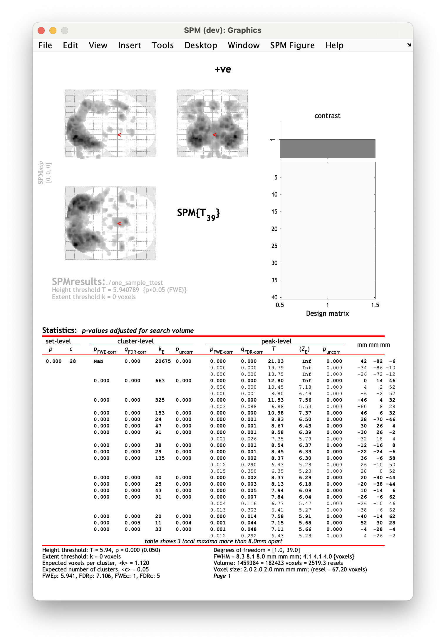
The SPM Graphics window shows you the activation map displayed on a glass brain (top left corner) shown in a standardised space with dark blobs representing clusters over the chosen threshold. You can also view your design matrix and the contrast you are currently viewing (top right corner). The bottom part of the results window, show summary statistics table for your results.
The columns in the results table show:
cluster-level- the chance (p) of finding a cluster with this many(kE) or a greater number of voxels, corrected (FWE or FDR)/uncorrected for search volume,peak-level- the chance (p) of finding (under the null hypothesis) a peak with this or a greater height (T- or Z-statistic), corrected (FWE or FDR)/uncorrected for search volume,x, y, z (mm)- coordinates in MNI space for each maximum.
You can also display your statistical maps on a different image. To do so, from the drop down menu in the SPM results window which shows overlays, select sections. In the pop-up, navigate to the folder where SPM is saved and select canonical/avg305T1.nii which is standard template in MNI space. This will display your results as a heatmap on a standard brain template: