Multimodal, Multisubject data fusion¶

fMRI Preprocessing and Statistics¶

We will keep description of the preprocessing and analysis of the fMRI data to a minimum, given that fMRI analysis is covered in several other chapters. We start with preprocessing Subject 15’s data. For the fMRI experiment, there were 9 runs (sessions), rather than the 6 in the M/EEG experiment. This is because the SOA was increased in the fMRI experiment, by virtue of jittering, which is necessary to estimate the BOLD response versus interstimulus baseline (e.g., to compare with the evoked EEG/MEG response versus prestimulus baseline). If you already launched SPM to analyse the M/EEG data from the previous sections, select “FMRI” instead of “EEG” in the pulldown menu of the main SPM window, otherwise start SPM by typing spm fmri. Preprocessing involves the following modules, which can be found under the menu “SPM – Spatial”:

Realignment of EPI (fMRI) data¶

The first step is to coregister the 9 runs of 208 images to one another (i.e., correcting for movement) using a rigid-body transform. Select “Realign: Estimate & Reslice”, and on the “Data” item, add nine new “Sessions”. Then, for the first session, select the 208 f*.nii images in the BOLD/Run_01 directory of Subject 15 (using right-click, “Select All”), and then repeat for the remaining eight sessions. On the “Reslice Options” item, change the default value of “All Images + Mean Image” to “Mean Image Only”. This is because we do not re-slice the EPI data: the coregistration parameters will be stored in the header information of the NIfTI file, and can be combined with the normalisation parameters when re-slicing the normalised images below (re-slicing can introduce interpolation artifacts so generally best to reduce number of re-slicings). However, we do need a re-sliced mean image, which we can use for coregistration with the T1 below. Thus the contents of the f*.nii files will change (as header updated), but no new (rf*.nii) files will be output, except for the meanf*.nii file.

Normalisation/Segmentation of T1 images¶

We will use SPM12’s unified segmentation to estimate normalisation parameters to MNI space. Select “Normalise: Estimate” item, add a new “Subject” in “Data” and select the mprage.nii image in the “SMRI” directory of Subject 15 for “Image to Align”. The output of this step will be a file y_mprage.nii containing the estimated deformation field that warps data from subject to MNI space.

Coregistration of mean EPI (fMRI) to T1 (sMRI)¶

Because we have determined the normalisation parameters from the subject’s native space to MNI space via the unified segmentation of their T1 image, we need to coregister all the EPI images to that T1 image, so that the normalisation warps can be later applied. Select “Coregister - Estimate” item, and for the “Reference Image”, select the same mprage.nii image in the SMRI directory. For the”Source Image”, select “Dependency” and then use “Realign: Estimate & Reslice: Mean Image”. For “Other Images”, select “Dependency” and then use the Ctrl key to select all 9 sessions from the “Realign” stage.

Application of Normalisation parameters to EPI data¶

We can now apply the normalisation parameters (warps) to each of the EPI volumes, to produce new, re-sliced wf images. Select “Normalise – Write” item, and for the “Deformation Field”, use select the “Normalise: Estimate: Deformation” dependency. For the “Images to Write”, select the “Coregister: Estimate: Coregistered Images”. You can also change the default voxel size from [2 2 2] to [3 3 3] if you want to save diskspace, since the original data are [3 3 3.9] (for Subject 15), so interpolation does not really gain new information.

Smoothing¶

Finally, we smooth the normalised images by an 8mm isotropic Gaussian kernel to produce swf* images. So select the “Smooth” item, and select the input to depend on the output of the prior “Normalisation: Write” stage.

Save batch and review¶

You can save this batch file (it should look like the batch_preproc_fmri_job.m file in the SPM12batch FTP directory), and then run it. You can inspect the realignment parameters, normalisations, etc. as described in other chapters. Make a new directory called Stats in the Sub15/BOLD directory.

Creating a 1st-level (fMRI) GLM¶

Select the “fMRI model specification” option from the “SPM – Stats” menu. Select the new Stats directory you created as the output directory. Set the “Units for design” to “seconds” (since our onsets files are in units of seconds) and the “interscan interval” (TR) to 2. Then under the “Data & Design” option, create a new Session, and then select all the swf*.nii images in the Run_01 directory as the “Scans”. Then under the “Multiple conditions” option, press “Specify” and select the file run_01_spmdef.mat that has been provided in the Trials sub-directory. This is a MATLAB file that contains the onsets, durations and names of every trial in Run1 (for this subject). Then under the “Multiple regressors” option, press “Specify” and select the file matching rp*.txt in the Run_01 directory. This is a text file that contains the 6 movement parameters for each scan, which was created during “Realignment” above, and we will add to the GLM to capture residual motion-related artifacts in the data.

For the basis functions, keep “Canonical HRF”, but change the “model derivatives” from “no” to “time and dispersion derivatives” (see earlier Chapter manuals). Then keep the remaining options as their defaults.

You then need to replicate this for the remaining 8 sessions, updating all three fields each time: i.e., the scans, conditions and (movement) regressors. It is at this point, that you might want to switch to scripting, which is much less effort – see e.g. this:

swd = '.../Sub15/BOLD'; % folder containing Subject 15's fMRI data
clear matlabbatch
matlabbatch{1}.spm.stats.fmri_spec.dir = {fullfile(swd,'Stats')};
matlabbatch{1}.spm.stats.fmri_spec.timing.units = 'secs';
matlabbatch{1}.spm.stats.fmri_spec.timing.RT = 2;
for r=1:9
    matlabbatch{1}.spm.stats.fmri_spec.sess(r).scans = ...
        cellstr(spm_select('FPList',fullfile(swd,sprintf('Run_%02d',r)),'^swf.*\.nii'));
    matlabbatch{1}.spm.stats.fmri_spec.sess(r).multi = ...
        cellstr(fullfile(swd,'Trials',sprintf('run_%02d_spmdef.mat',r)));
    matlabbatch{1}.spm.stats.fmri_spec.sess(r).multi_reg = ...
        cellstr(spm_select('FPList',fullfile(swd,sprintf('Run_%02d',r)),'^rp_.*\.txt'));
end
matlabbatch{1}.spm.stats.fmri_spec.bases.hrf.derivs = [1 1];
spm_jobman('interactive',matlabbatch);

Model Estimation¶

Add a module for “Model estimation” from the “SPM – Stats” menu and define the SPM.mat file name as being dependent on the results of the fMRI model specification output. For “write residuals”, keep “No” and stick to “Classical” estimation.

Setting up contrasts¶

To create some contrasts, select “Contrast Manager” from the “SPM – Stats” menu. Define the SPM.mat file name as dependent on the model estimation. The first contrast will be a generic one that tests whether significant variance is captured by the 3 canonical HRF regressors (one per condition). So create a new F-contrast, call it the “Canonical HRF effects of interest”, and enter as the weights matrix (SPM will automatically perform zero padding over the movement regressors):

   [1 0 0 0 0 0 0 0 0
    0 0 0 1 0 0 0 0 0
    0 0 0 0 0 0 1 0 0]

Then select “Replicate” to reproduce this across the 9 sessions. We can also define a T-contrast to identify face-related activation, e.g., “Faces \(>\) Scrambled Faces”, given the weight matrix [0.5 0 0 0.5 0 0 -1 0 0], again replicated across sessions. (Note that there are 3 basis functions per condition, and the zeros here ignore the temporal and dispersion derivatives, but if you want to include them, you can add them as separate rows and test for any face-related differences in BOLD response with an F-contrast; see earlier chapters).

Finally, for the group-level (2nd-level) analyses below, we need an estimate of activation of each condition separately (versus baseline), averaged across the sessions. So create three new T-contrasts, whose weights correspond to the three rows of the above F-contrast, i.e, that pick out the parameter estimate for the canonical HRF (with “Replicate over sessions” set to “Replicate”):

for Famous: [1 0 0 0 0 0 0 0 0],
for Unfamiliar: [0 0 0 1 0 0 0 0 0],
for Scrambled: [0 0 0 0 0 0 1 0 0].

These T-contrasts will be numbered 3-5, and used in group analysis below.[^4]

Save batch and review¶

You can save this batch file (it should look like the batch_stats_fmri_job.m file in the SPM12batch FTP directory). When it has run, you can press “Results” from the SPM Menu window, select the SPM.mat file in the BOLD directory, and explore some of the contrasts. However, we will wait for the group analysis below before showing results here.

Creating a script for analysis across subjects¶

Now that we have created a pipeline for fMRI preprocessing and analysis for a single subject, we can script it to run on the remaining 15 subjects. Below is an example from the master_script.m:

nrun = 9;

spm_jobman('initcfg');
spm('defaults', 'FMRI');
for s = 1:nsub

    %% Change to subject's directory
    swd = fullfile(outpth,subdir{s},'BOLD');
    cd(swd);

    %% Preprocessing
    jobfile = {fullfile(scrpth,'batch_preproc_fmri_job.m')};
    inputs  = cell(nrun+2,1);
    for r = 1:nrun
        inputs{r} = cellstr(spm_select('FPList',fullfile(outpth,subdir{s},'BOLD',sprintf('Run_%02d',r)),'^fMR.*\.nii$'));
    end   
    inputs{10} = cellstr(spm_select('FPList',fullfile(outpth,subdir{s},'SMRI'),'^mprage.*\.nii$'));
    inputs{11} = cellstr(spm_select('FPList',fullfile(outpth,subdir{s},'SMRI'),'^mprage.*\.nii$'));
    spm_jobman('serial', jobfile, '', inputs{:});

    %% 1st-level stats
    jobfile = {fullfile(scrpth,'batch_stats_fmri_job.m')};
    inputs  = {}; %cell(nrun*3+1,1);
    inputs{1} = {fullfile(swd,'Stats')}; 
    try mkdir(inputs{1}{1}); end
    for r = 1:nrun
        inputs{end+1} = cellstr(spm_select('FPList',fullfile(outpth,subdir{s},'BOLD',sprintf('Run_%02d',r)),'^swfMR.*\.nii$'));
        inputs{end+1} = cellstr(fullfile(outpth,subdir{s},'BOLD','Trials',sprintf('run_%02d_spmdef.mat',r)));
        inputs{end+1} = cellstr(spm_select('FPList',fullfile(outpth,subdir{s},'BOLD',sprintf('Run_%02d',r)),'^rp.*\.txt$'));
    end   
    spm_jobman('serial', jobfile, '', inputs{:});

    eval(sprintf('!rm -r %s/Run*/f*',swd)) % to save diskspace (take care!)
    eval(sprintf('!rm -r %s/Run*/wf*',swd)) % to save diskspace (take care!)
end

(The last two lines in the loop are optional, to delete intermediate files and save diskspace.) Once you have run this script, we can do 2nd-level (group) statistics on resulting contrast images for each condition (averaged across 9 runs).

Group Statistics on fMRI data¶

Now we have a new set of 16\(\times\)3 NIfTI images for each subject and each condition, we can put them into the same repeated-measures ANOVA that we used to test for differences in power across sensors in the time-frequency analysis above, i.e, re-use the batch_stats_rmANOVA_job.m file created above. This can be scripted as:

fmristatsdir = fullfile(outpth,'BOLD');
if ~exist(fmristatsdir)
    eval(sprintf('!mkdir %s',fmristatsdir));
end

jobfile = {fullfile(scrpth,'batch_stats_rmANOVA_job.m')};

inputs  = cell(nsub+1, 1);
inputs{1} = {fmristatsdir};
for s = 1:nsub
    inputs{s+1,1} = cellstr(strvcat(spm_select('FPList',fullfile(outpth,subdir{s},'BOLD','Stats'),'con_000[345].nii')));   % Assumes that these T-contrasts in fMRI 1st-level models are famous, unfamiliar, scrambled (averaged across sessions)
end

spm_jobman('serial', jobfile, '', inputs{:});

Save batch and review.¶

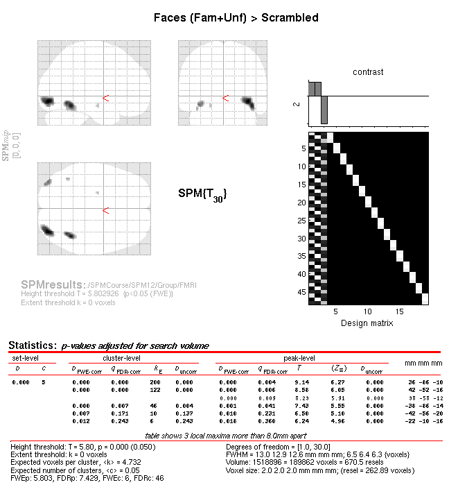
When the script has run, press “Results” from the SPM Menu window and select the SPM.mat file in the BOLD directory. From the Contrast Manager window, select the pre-specified T-contrast “Faces (Fam+Unf) \(>\) Scrambled”. Within the “Stats: Results” window, when given the option, select the following: Apply Masking: None, P value adjustment to control: FWE, keep the threshold at 0.05, extent threshold voxels: 0; Data Type: Volumetric 2D/3D. The Graphics window should then show what is in Figure 1.11 below. Note the left and right OFA and FFA (more extensive on right), plus a small cluster in left medial temporal lobe.

*Group SPM for Faces vs Scrambled fMRI data at p < .05 FWE-corrected.*

Later, we can use these five clusters as priors for constraining the inversion of our EEG/MEG data. To do this, we need to save these as an image. Press the “save...” button in the bottom right of the SPM Results window, and select the “all clusters (binary)” option. The window will now prompt you for an output filename, in which you can type in fac-scr_fmri_05_cor. This image will be output in the BOLD directory, and we will use it later.