Multimodal, Multisubject data fusion
Source Reconstruction
To estimate the cortical sources that give rise to the EEG and MEG data, we will return to Subject 15, in order to demonstrate forward and inverse modelling. We need to use the structural MRI of the subject to create a “head model” (that defines the cortex, skull and scalp in terms of meshes) and then a “forward model” (that uses a conductor model to simulate the signal at each sensor predicted by a dipolar source at each point in the cortical mesh). This corresponds to an “imaging” or “distributed” solution to the “Inverse problem”, but you should note that SPM offers other inverse solutions, such as a Bayesian implementation of Equivalent Current Dipoles, and also DCM, which can be viewed as a type of inverse solution (see other chapters in this manual).
You can view the structural MRI of Subject 15 by displaying the NIfTI
file mprage.nii in the SMRI (T1) sub-directory. This image was
manually positioned to roughly match Talairach space, with the origin
close to the Anterior Commissure. The approximate position of 3
fiducials within this MRI space – the nasion, and the left and right
pre-auricular points – are stored in the file mri_fids.mat. These
were identified manually (based on anatomy) and are used to define the
MRI space relative to the EEG and MEG spaces, which need to be
coregistered (see below).
To estimate total power (evoked and induced) of the cortical sources, we
need to have the original data for each individual trial. Therefore our
input file will be apMcbdspmeeg_run_01_sss.mat (we could select the
trial-averaged file if we just wanted to localise evoked effects). Note
that one cannot localise power (or phase) data directly, nor can one
localise RMS data from combined gradiometers.
Create Head Model
Select the source reconstruction option in the batch window, and select
“Head model specification”. Select the file
apMcbdspmeeg_run_01_sss.mat as the “M/EEG datasets”, and the inversion
index as 1 (this index can track different types of forward models and
inverse solutions, for example if you want to compare them in terms of
log-evidence, e.g., Henson et al, 2009). Additional comments relating to
each index can be inserted if “comments” is selected.
The next step is to specify the meshes. Highlight “meshes” and select
“mesh source”. From here select “Individual structural image” and select
the mprage.nii in the SMRI directory. The mesh resolution can be
kept as normal (approximately 4000 vertices per hemisphere). Note that
the cortical mesh (and scalp and skull meshes) are created by warping
template meshes from a brain in MNI space, based on normalising this
subject’s MRI image to that MNI brain (see papers on “canonical” meshes
in SPM).
To coregister the MRI and MEEG data, you must select “specify
coregistration parameters”. First you need to specify the select
fiducials. You will need to select at least three of these, with
coordinates in the space of the MRI image selected. Here we will define
“Nasion”; “LPA”; “RPA”. You can do this by loading the MRI and clicking,
but here we will use the coordinates provided in the mri_fids.mat file
described above. You can view these coordinates by loading that file
into MATLAB, but we repeat them below for convenience. For the Nasion,
select “type MRI coordinates” and enter: [4 112 1]; for LPA, enter
[-80 21 -12]; for RPA, enter [79 9 -31].
As well as the fiducials, a number of “head-points” across the scalp were digitised. These were read from the FIF file and stored in the SPM MEEG file. These can help coregistration, by fitting them to the scalp surface mesh (though sometimes they can distort coregistration, e.g. if the end of the nose is digitised, since the nose does not appear on the scalp mesh, often because it has poor contrast on T1-weighted MRI images). If you keep “yes” for the “use headshape points” option, these points will be used, but you will notice that alignment of the fiducials is not as good (as if you don’t use the headshape points), most likely because the nose points are pulling it too far forward. So here we will say “no” to the “use headshape points” option, so as to rely on the fiducials alone, and trust the anatomical skills of the experimenter. (Alternatively, you could edit the headpoints via the command line or a script so as to remove inappropriate ones, but we will not go into the details here).
Finally, for the forward model itself, select “EEG head model”, and specify this as “EEG BEM”; select “MEG head model” and specify this as “Single Shell”. This can then be run. Note that the model parameters are saved, but the gain matrix itself is not estimated until inversion.
Save batch and review.
You can now save this inversion batch file (it should look like the
batch_localise_forward_model_meeg_job.m file in the SPM12batch FTP
directory). Once you have run it, you can explore the forward model by
pressing the “3D Source Reconstruction” button within the SPM Menu
window. This will create a new window, in which you can select “Load”
and choose the apMcbdspmeeg_run_01_sss.mat file. On the left hand side
of the “source localisation” window, select the “display” button below
the “MRI” button. This will bring up the scalp (orange), inner and outer
skull (red) and cortical (blue) meshes of Subject 15’s brain, like in
Figure 1.12 (left, after rotating slightly
with MATLAB ‘s 3D tool). Note that the fiducials are shown by cyan
disks.
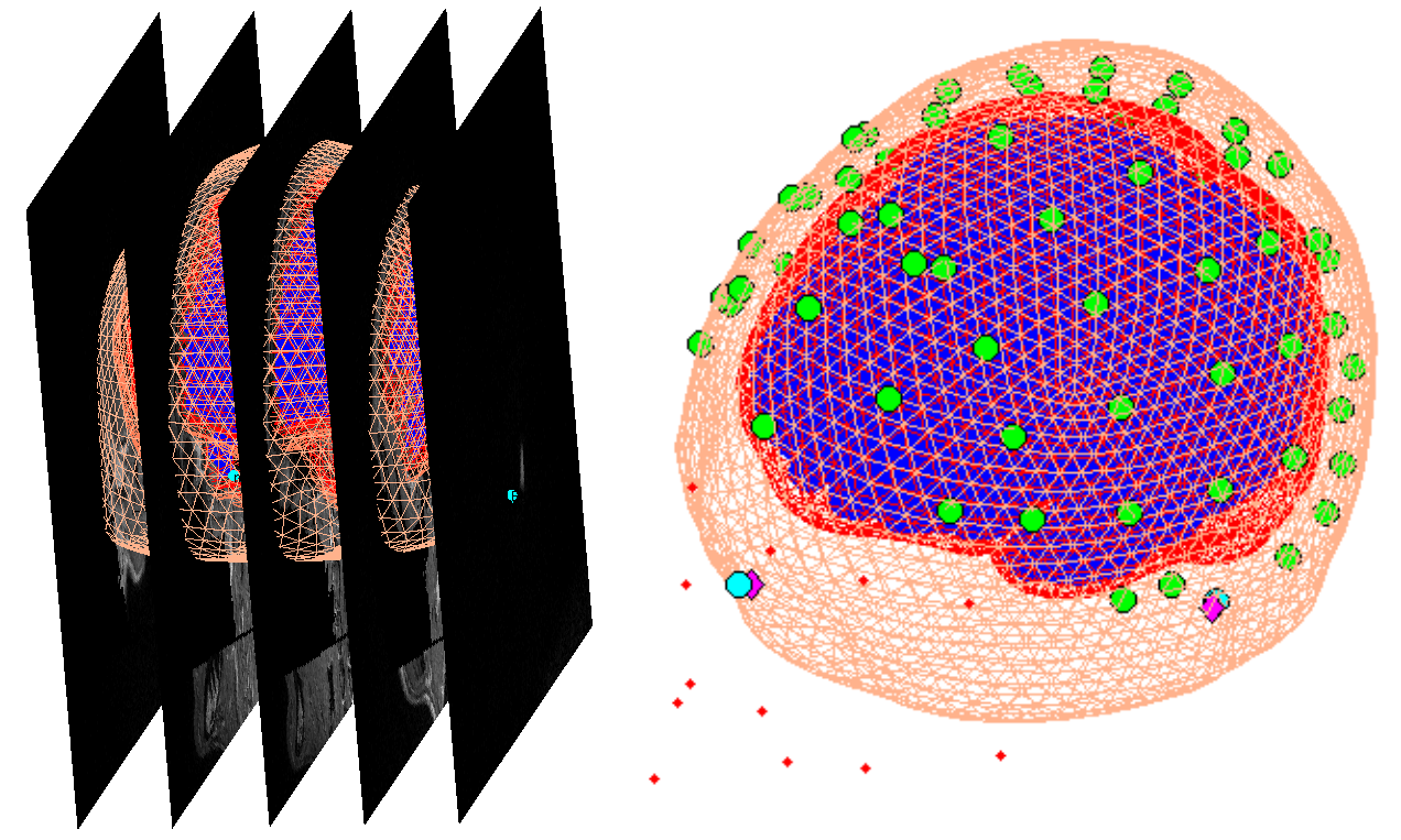
Next, select the “display” button beneath “Co-register” and then select “EEG” when asked what to display. The Graphics window should then display an image like in Figure 12 (right) that displays the electrode locations in green disks, the digitized headpoints in small red dots, the fiducials in the EEG data as purple diamonds, and the MRI fiducials as cyan disks again. The overlap between the EEG fiducials and MRI fiducials indicates how well the data have been coregistered (assuming no error in marking these anatomical features).
Finally, select “Display” located beneath “Forward Model” and this time select “EEG”. You should see an image displaying the EEG electrode locations relative to the four meshes.
Model Inversion
We will compare two approaches to inverting the above forward model
(both within a Parametric Empirical Bayesian framework). The first one
is called “Multiple Sparse Priors”, which is a novel approach unique to
SPM. This corresponds to a sparse prior on the sources, namely that only
a few are active. Go back to the batch editor, and select “M/EEG –
Source reconstruction – Source Inversion”. Select the same input file
apMcbdspmeeg_run_01_sss.mat, and set the inversion index to 1.
Highlight “what conditions to include” and select “All”. Next highlight
inversion parameters, choose “custom” and set the inversion type to
“GS”. This is one of several fitting algorithms for optimising the MSP
approach: Greedy Search (GS), Automatic Relevance Detection (ARD) and
GS+ARD. We choose GS here because it is quickest and works well for
these data. Then enter the time window of interest as [-100 800]. Set
the frequency window of interest to [0 256]. Select “yes” for the “PST
Hanning window”. Keep all the remaining parameters at their defaults,
including the Modalities as “All” (which will simultaneously invert, or
“fuse”, the data from the EEG, magnetometers and gradiometers [Henson
et al, 2009]).
The second type of inversion we will examine corresponds to a L2-minimum
norm (MNM), i.e, fitting the data at the same time as minimising the
total energy of the sources. In SPM, this is called “IID” because it
corresponds to assuming that the prior probability of each source being
active is independent and identically distributed (i.e., an identity
matrix for the prior covariance). Go back to the batch editor, add
another “M/EEG – Source reconstruction – Source Inversion” module, and
select the same input files as before (apMcbdspmeeg_run_01_sss.mat),
but this time set the inversion index to 2. Set the inversion
parameters to “custom”, but the inversion type to be “IID”. The
remaining parameters should be made to match the MSP (GS) inversion
above.
Time-frequency contrasts
Here we are inverting the whole epoch from -100 to +800ms (and all
frequencies), which will produce a timecourse for every single source.
If we want to localise an effect within the cortical mesh, we need to
summarise this 4D data by averaging power across a particular
time-frequency window. To do this, select “M/EEG – Source
reconstruction – Inversion Results”. Specify the input as dependent on
the output of the source inversion, and set the inversion index to 1.
Based on the results of the group sensor-level time-frequency analyses
in the previous section, set the time window of interest to [100 250]
and the frequency window of interest to [10 20]. For the contrast
type, select “evoked” from the current item window, and the output space
as “MNI”. Then replicate this module to produce a second “inversion
results” module, simply changing the index from 1 to 2 (i.e. to
write out the time-frequency contrast for the MNM (IID) as well as MSP
(GS) solution).
Now the source power can be written in one of two ways: 1) either as a
volumetric NIfTI “Image”, or as 2) a surface-based GIfTI “Mesh”. The
source data are currently represented on the cortical mesh, so writing
them to a volumetric image involves interpolation. If we chose this, we
could treat the resulting contrast images in the same way that we do MRI
images, and use 3D Random Field Theory (RFT) for voxel-wise statistics.
This is likely to require considerable 3D smoothing however, to render
the interpolated cortical surface more suitable for RFT. This is what
was done in SPM8. However, in SPM12, RFT can also be applied to 2D
surfaces (that live in a 3D space), in which case we can restrict
smoothing to a small amount across the surface (rather than volume),
which is closer to the nature of the data. Therefore, we will chose
“Mesh” here to write out GifTI surfaces (which are also much smaller in
filesize), keeping the default cortical smoothing of 8.
Save batch and review
You can now save this inversion batch file (it should look like the
batch_localise_evoked_job.m file in the SPM12batch FTP directory).
It will take a while to run (because it has to create the gain matrix
for the first time), after which you can review the inverse results from
within the same “3D Source Reconstruction” interface that you used to
examine the forward model above. You have to re-“Load” the
apMcbdspmeeg_run_01_sss.mat file. The latest inversion index will be
shown (2 in this case), which corresponds to the IID inversion. Press
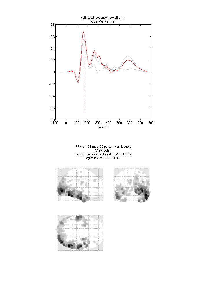
the “mip” button below the “Invert” button, and you should see something
like Figure 1.13. The top plot shows the evoked
responses for the three conditions from the peak vertex (at +52 -59 -21,
i.e. right fusiform) at 165ms, with the red line being the currently
selected condition, here “1” for Famous faces (press the “condition”
button to toggle through the other conditions). If you press “display”
under the “Window” button, you can see a MIP for the time-frequency
contrast limited to the 100-250ms, 10-20Hz specified above, or if you
press the “display” under the “Image” button, you will see a rendered
version.
If you press the “previous” button, you can select the previous inversion (1), which here corresponds to the MSP inversion. Press the “mip” button again, and you should see results that are sparser and deeper inside the brain, in medial and anterior temporal cortex. This solution actually has a higher model evidence (even though it explains a smaller % of the data variance) because it corresponds to a less complex model (i.e, the posterior deviates less from the prior). We will compare these two inverse solutions in a different way when we do group statistics below.
If you like, you can also explore other inversion options, either with
batch or with this reconstruction window (e.g., creating new inversion
indices, though keep in mind that the associated
apMcbdspmeeg_run_01_sss.mat file can get very large). For example, you
can compare localisation of EEG data alone, or Magnetometers alone, etc.
Creating a script for analysis across subjects
Now that we have created a pipeline for forward and inverse modelling,
we can script it to run on the remaining 15 subjects. Below is an
example from the master_script.m:
for s = 1:nsub

    %% Change to subject's directory
    swd = fullfile(outpth,subdir{s},'MEEG');
    cd(swd);

    jobfile = {fullfile(scrpth,'batch_localise_forward_model_meeg_job.m')};
    inputs  = cell(5,1);
    inputs{1} = cellstr(spm_select('FPList',fullfile(outpth,subdir{s},'MEEG'),'^apMcbdspmeeg.*\.mat$'));
    inputs{2} = cellstr(spm_select('FPList',fullfile(outpth,subdir{s},'SMRI'),'^mprage.*\.nii$'));
    f = load(spm_select('FPList',fullfile(outpth,subdir{s},'SMRI'),'^mri_fids.*\.mat$'));
    inputs{3} = f.mri_fids(1,:);
    inputs{4} = f.mri_fids(2,:);
    inputs{5} = f.mri_fids(3,:);
    spm_jobman('serial', jobfile, '', inputs{:});

    %% MSP inversion of EEG, MEG, MEGPLANAR, ALL, then IID inversion of ALL and a time-freq contrast
    jobfile = {fullfile(scrpth,'batch_localise_evoked_job.m')};
    inputs = cell(1,4);
    inputs{1} = cellstr(spm_select('FPList',fullfile(outpth,subdir{s},'MEEG'),'^apMcbdspmeeg.*\.mat$'));
    inputs{2} = {''};  % No fMRI priors
    inputs{3} = cellstr(spm_select('FPList',fullfile(outpth,subdir{s},'MEEG'),'^apMcbdspmeeg.*\.mat'));
    inputs{4} = {''};  % No fMRI priors
    spm_jobman('serial', jobfile, '', inputs{:});
end
Once you have run this script, we can do statistics on the source power GIfTI images created for each subject (using the same repeated-measures ANOVA model that we used for the time-frequency sensor-level analyses above).
Group Statistics on Source Reconstructions
Once we have the 16\(\times\)3 GIfTI images for the power between
10-20Hz and 100-250ms for each subject for each condition, we can put
them into the same repeated-measures ANOVA that we used above, i.e. the
batch_stats_rmANOVA_job.m file. We actually want to do two ANOVAs: one
for the MSP inversion and one for the MNM inversion. So we can again
script this, like below:
srcstatsdir{1} = fullfile(outpth,'MEEG','IndMSPStats');
srcstatsdir{2} = fullfile(outpth,'MEEG','IndMNMStats');

jobfile = {fullfile(scrpth,'batch_stats_rmANOVA_job.m')};

for val = 1:length(srcstatsdir)
    if ~exist(srcstatsdir{val})
        eval(sprintf('!mkdir %s',srcstatsdir{val}));
    end

    inputs  = cell(nsub+1, 1);
    inputs{1} = {srcstatsdir{val}};
    for s = 1:nsub
        inputs{s+1,1} = cellstr(strvcat(spm_select('FPList',fullfile(outpth,subdir{s},'MEEG'),sprintf('^apMcbdspmeeg_run_01_sss_%d.*\.gii$',val))));
    end

    spm_jobman('serial', jobfile, '', inputs{:});
end
where the “Ind” in the output directories refers to “individual” source reconstructions, in contrast to the group-based reconstructions we will do below.
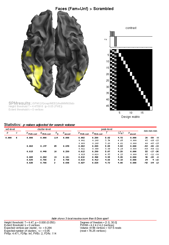
When it has run, press “Results” from the SPM Menu window an select the
SPM.mat file in the MEEG/IndMNMStats directory to look at the
results of the minimum norm inversion. From the Contrast Manager window,
select the pre-specified T-contrast “Faces (Fam+Unf) \(>\) Scrambled”.
Within the “Stats: Results” window, select the following: Apply Masking:
None, P value adjustment to control: FWE, keep the threshold at 0.05,
extent threshold voxels: 0; Data Type: Volumetric 2D/3D. The Graphics
window should then show what is in
Figure 1.14 below (after having right-clicked
on the rendered mesh, selecting “View” and then “x-y view (bottom)”, in
order to reveal the underside of the cortex). Note the broad right
fusiform cluster, with additional clusters on left and more anteriorly
on right. You can compare this to the fMRI group results in the previous
section.
You can also look at the results of the MSP inversion by selecting the
SPM.mat file in the MEEG/IndMSPStats directory. This will not reveal
any face-related activations that survive \(p<.05\) FWE-corrected. The
likely reason for this is that the sparse solutions for each individual
subject are less likely to overlap at the group level (than the
“smoother” minimum-norm solution). If you change the threshold to
\(p<.001\) uncorrected, you will see some activation in posterior right
fusiform. However, we can improve the MSP reconstructions by pooling
across subjects when actually inverting the data – so-called “group
inversion” that we consider next.
Group Source Reconstruction
Because of the indeterminacy of the inverse problem, it is helpful to provide as many constraints as possible. One constraint is to assume that every subject has the same underlying source generators, that are simply seen differently at the sensors owing to different anatomy (head models) and different positions with respect to the sensors (forward models). In the PEB framework, this corresponds to assuming the same set of source priors across subjects (allowing for different sensor-level noise; see [Henson et al, 2011]). This group-based inversion can be implemented in SPM simply by selecting multiple input files to the inversion routine, which can be scripted like this (using the same batch file as before, noting that this includes two inversions – MNM and MSP – hence the two inputs of the same data files below):
Note that once you have run this, the previous “individual” inversions
in the data files will have been overwritten (you could modify the batch
to add new inversion indices 3 and 4, so as to compare directly the
group inversions with the previous individual inversions, but the files
will get very big).
Group Statistics on Source Reconstructions
Now we have a new set of 16\(\times\)3 GIfTI images for the power
between 10-20Hz and 100-250ms for each subject for each condition after
group-inversion, we can put them into the same repeated-measures ANOVA
that we used above, i.e., the batch_stats_rmANOVA_job.m file. This can
be scripted as (i.e, simply changing the output directories at the start
from, e.g, IndMSPStats to GrpMSPStats).
srcstatsdir{1} = fullfile(outpth,'MEEG','GrpMSPStats');
srcstatsdir{2} = fullfile(outpth,'MEEG','GrpMNMStats');

jobfile = {fullfile(scrpth,'batch_stats_rmANOVA_job.m')};

for val = 1:length(srcstatsdir)
    if ~exist(srcstatsdir{val})
        eval(sprintf('!mkdir %s',srcstatsdir{val}));
    end

    inputs  = cell(nsub+1, 1);
    inputs{1} = {srcstatsdir{val}};
    for s = 1:nsub
        inputs{s+1,1} = cellstr(strvcat(spm_select('FPList',fullfile(outpth,subdir{s},'MEEG'),sprintf('^apMcbdspmeeg_run_01_sss_%d.*\.gii',val))));
    end

    spm_jobman('serial', jobfile, '', inputs{:});
end
When it has run, press “Results” from the SPM Menu window and select the
SPM.mat file in the relevant output directories. You will notice that
the results for minimum norm have not changed much – a lot of voxels
remain significant after correction, but in a broadly distributed swathe
of ventral temporal lobe. For the results in the MEEG/GrpMSPStats
directory, there is a small anterior right temporal cluster that
survives correction. But if you lower the threshold to \(p<.001\)
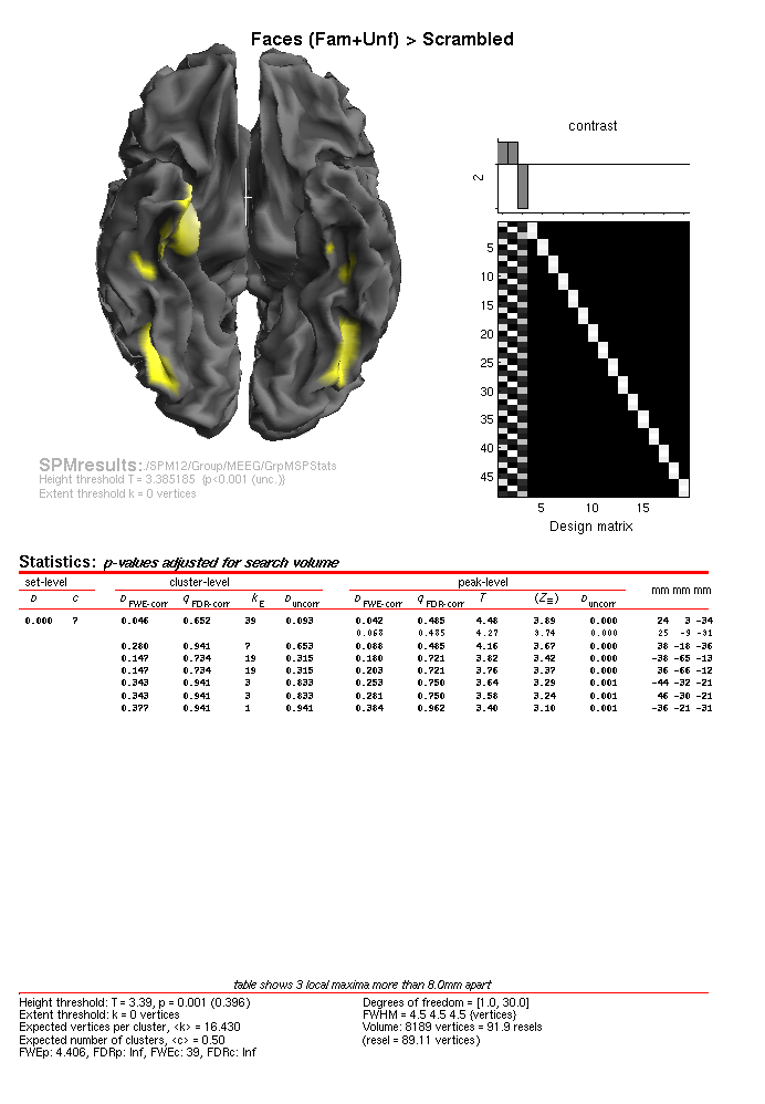
uncorrected, you should see results like in
Figure 1.15, which includes more focal
regions in the ventral temporal lobe, and importantly, more such regions
that for the individual MSP inversions the MEEG/IndMSPStats directory
(demonstrating the advantage of group-based inversion).
Group MEEG Source Reconstruction with fMRI priors
Finally, in an example of full multi-modal integration, we will use the significant clusters in the group fMRI analysis as separate spatial priors for the group-optimised source reconstruction of the fused MEG and EEG data (see [Henson et al, 2011]). Each cluster becomes a separate prior, allowing for fact that activity in those clusters may occur at different post-stimulus times.
This group-based inversion can be implemented in SPM simply by selecting
the binary (thresholded) image we created from the group fMRI statistics
(fac-scr_fmri_05_cor.nii in the BOLD directory), which contains
non-zero values for voxels to be included in the clustered priors. This
is simply an option in the inversion module, so can scripted like this
(using the same batch file as before, noting that this includes two
inversions – MNM and MSP – hence the two inputs of the same data files
below):
jobfile = {fullfile(scrpth,'batch_localise_evoked_job.m')};
tmp = cell(nsub,1);
for s = 1:nsub
    tmp{s} = spm_select('FPList',fullfile(outpth,subdir{s},'MEEG'),'^apMcbdspmeeg.*\.mat');
end
inputs = cell(4,1);
inputs{1} = cellstr(strvcat(tmp{:}));
inputs{2} = {fullfile(outpth,'BOLD','fac-scr_fmri_05cor.nii')};  % Group fMRI priors
inputs{3} = cellstr(strvcat(tmp{:}));
inputs{4} = {fullfile(outpth,'BOLD','fac-scr_fmri_05cor.nii')};  % Group fMRI priors
spm_jobman('serial', jobfile, '', inputs{:});
Note again that once you have run this, the previous “group” inversions
in the data files will have been overwritten (you could modify the batch
to add new inversion indices 5 and 6, so as to compare with previous
inversions above, but the file will get very big). Note also that we
have used group-defined fMRI priors, but the scripts can easily be
modified to define fMRI clusters on each individual subject’s 1st-level
fMRI models, and use subject-specific source priors here.
Group Statistics on Source Reconstructions
After running the attached script, we will have a new set of
16\(\times\)3 GIfTI images for the power between 10-20Hz and
100-250ms for each subject for each condition after group-inversion
using fMRI priors, and can put them into the same repeated-measures
ANOVA that we used above, i.e. the batch_stats_rmANOVA_job.m file.
This can be scripted as (i.e. simply changing the output directories at
the start from, e.g. GrpMNMStats to fMRIGrpMNMStats).
srcstatsdir{1} = fullfile(outpth,'MEEG','fMRIGrpMSPStats');
srcstatsdir{2} = fullfile(outpth,'MEEG','fMRIGrpMNMStats');

jobfile = {fullfile(scrpth,'batch_stats_rmANOVA_job.m')};

for val = 1:length(srcstatsdir)
    if ~exist(srcstatsdir{val})
        eval(sprintf('!mkdir %s',srcstatsdir{val}));
    end

    inputs  = cell(nsub+1, 1);
    inputs{1} = {srcstatsdir{val}};
    for s = 1:nsub
        inputs{s+1,1} = cellstr(strvcat(spm_select('FPList',fullfile(outpth,subdir{s},'MEEG'),...
            sprintf('^apMcbdspmeeg_run_01_sss_%d.*\.gii$',val))));
    end

    spm_jobman('serial', jobfile, '', inputs{:});
end
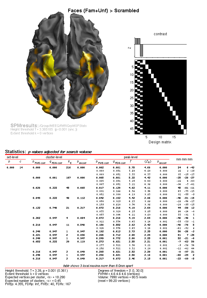
When it has run, press “Results” from the SPM Menu window an select the
SPM.mat file from the fMRIGrpMSPStats directory, and choose an
uncorrected threshold of \(p<.001\). You should see results like in
Figure 1.16, which you can compare to
Figure 1.15. The fMRI priors have improved
consistency across subjects, even in medial temporal lobe regions, as
well as increasing significance of more posterior and lateral temporal
regions (cf., Figure 1.11, at \(p<.001\) uncorrected).