Analysis
If you have got to this stage, then hopefully in every subjects folder you have a swm[tissue-class][filename].nii.
Before we construct a model, we will need one additional covariate in addition to those we already have for our study population – total intracranial volume
In SPM, there is a function to do this. Open the batch menu, select SPM Util Tissue volumes.
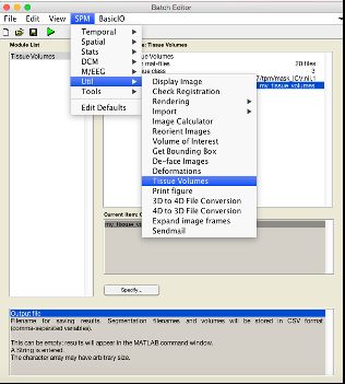
You will need to input the seg8.mat from the segmentation steps earlier. Recursively search using .*seg8.mat.

It will either output in MATLAB prompt, or if you specify a file it will generate a .csv you can use in excel. You will need to sum the three tissue classes (GM, WM, CSF) to obtain a volume in litres for each subject.
Model
First make a new directory for your specific analysis. You will need one directory for each analysis you do.
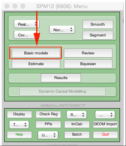
Then from the SPM menu, select Basic models.
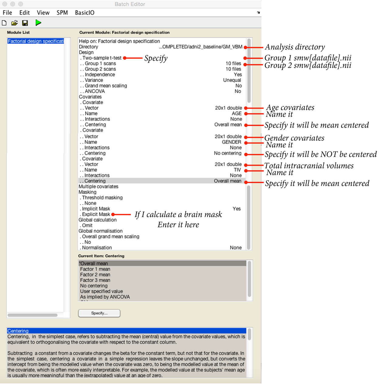
The precise set-up will depend on your study. Over I have provided an example for a two-sample t-test, controlling for age, gender and total intracranial volume.
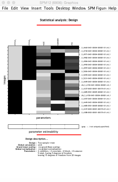
Again save your batch before proceeding. If you have done everything right, you will see the design matrix corresponding to your model (see next page). Now select Estimate from the SPM menu, select the SPM.mat in the folder you are using, and hit go.

Analysis and visualisation
Before we finish, it is a good idea to generate a population average brain for projecting our data onto (because it is not precisely MNI). To do this, we simply warp the intensity nonuniformity corrected T1s to our group average space. You can do this using SPM Tools Shoot tools Write normalised
-
Shoot Template: As before, select the final template image created in the previous step (
Template_4.nii). -
Select according to: Choose Many Subjects.
-
Many Subjects
-
Deformation fields: Select all the
y_*.nii. -
Images: Need one channel of images for warping the intensity nonuniformity corrected scans.
- Images: Select the intensity nonuniformity corrected images (
m*.nii), in the same order as the deformation fields.
- Images: Select the intensity nonuniformity corrected images (
-
-
-
Voxel Sizes: Specify voxel sizes for spatially normalised images (1mm might be a good choice).
-
Bounding box: The field of view to be included in the spatially normalised images can be specified here. For now though, just leave at the default settings.
-
Preserve: For warping images, this should be set to Preserve concentrations (no “modulation”).
-
Gaussian FWHM: We don’t want to smooth, so choose 0 mm.
All being well, this will generate a w[filename].nii in each folder.
Now to generate an average image, select Imcalc from the SPM menu:
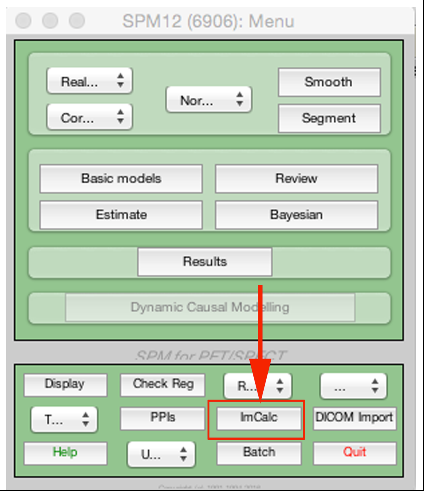
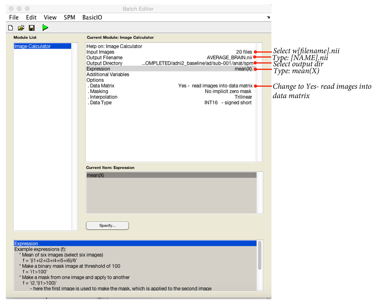
This will read in all the w[filenames].nii and calculate a population average:
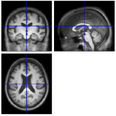
Now onto looking at our results:
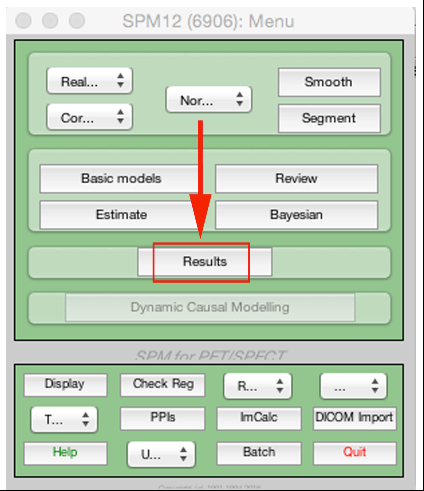
This will open a file select, you need to go to your analysis folder and pick the SPM.mat. Following this, the contrast manager will open. Click Define new contrast.
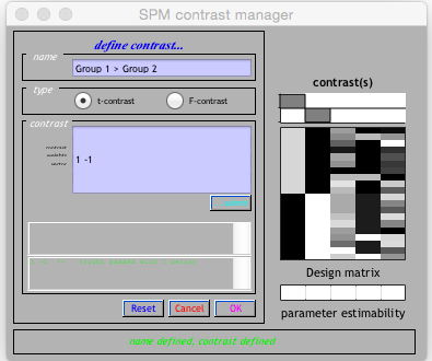
Enter a name.
To test for regions of the brain significantly bigger in group 1 vs. group 2, enter 1 -1 into the contrast, then click Ok. To do the opposite analysis (group 2 regions > group 1) enter -1 1.
Then:
Apply maskingNone(or enter a mask if you have one)CorrectionFWEP value0.05Extent threshold0
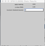
The next window displays any results that survive FWE correction at P < 0.05, displayed on a glass brain.
If you want to see these results on an actual MRI, click (overlay) and select sections and then input the average brain you just calculated.
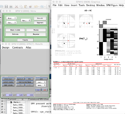
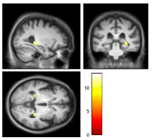
If you want to change the contrast, or inspect a different threshold (P < 0.001 uncorrected), use the Contrasts menu.
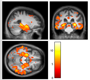
You can save your thresholded SPM result in the save menu (the one under the overlay menu). You can then use your data visualization program of choice to generate results.